Signals and Systems Chapter 1 Problems Part 1 (1.1-1.20)

- 1 Problem 1.1
- 2 Problem 1.2
- 3 Problem 1.3
- 4 Problem 1.4
- 5 Problem 1.5
- 6 Problem 1.6
- 7 Problem 1.7
- 8 Problem 1.8
- 9 Problem 1.9
- 10 Problem 1.10
- 11 Problem 1.11
- 12 Problem 1.12
- 13 Problem 1.13
- 14 Problem 1.14
- 15 Problem 1.15
- 16 Problem 1.16
- 17 Problem 1.17
- 18 Problem 1.18
- 18.1 linearity
- 18.2 time invariant
- 18.3 find \(C\)
- 19 Problem 1.19
- 20 Problem 1.20
1 Problem 1.1
Problem 1.1: Express each of the following complex numbers in Cartesian form \(x+iy\):
\begin{equation*}
\begin{array}{ccc}
\frac{1}{2}e^{i\pi} & \frac{1}{2}e^{-i\pi} & e^{i\pi/2} \\
e^{-i\pi/2} & e^{i5\pi/2} & \sqrt{2}e^{i\pi/4} \\
\sqrt{2}e^{i9\pi/4} & \sqrt{2}e^{-i9\pi/4} & \sqrt{2} e^{-i\pi/4}
\end{array}
\end{equation*}
First, let’s figure them out using the Euler’s formula. For the nine complex numbers in Problem 1.1, we have:
\begin{eqnarray*}
\tfrac{1}{2} e^{i\pi } &=& \tfrac{1}{2} (\cos(\pi) + i\sin(\pi) ) = \tfrac{1}{2} \cos(\pi) = -\tfrac{1}{2} \\
\tfrac{1}{2} e^{-i\pi} &=& \tfrac{1}{2} (\cos(-\pi) + i\sin(-\pi) ) = \tfrac{1}{2} \cos(-\pi) = -\tfrac{1}{2} \\
e^{i\pi/2} &=& \cos(\pi/2) + i \sin(\pi/2) = i \\
e^{-i\pi/2} &=& \cos(-\pi/2) + i \sin(-\pi/2) = -i \\
e^{i5\pi/2} &=& \cos(5\pi/2) + i \sin(5\pi/2) = \cos(2\pi + \pi/2) + i \sin(2\pi + \pi/2) = i \sin(\pi/2) = i \\
\sqrt{2}e^{i\pi/4} &=& \sqrt{2} ( \cos(\pi/4) + i \sin(\pi/4) ) = \sqrt{2} ( \tfrac{\sqrt{2}}{2} + i\tfrac{\sqrt{2}}{2} ) = 1 + i \\
\sqrt{2} e^{i9 \pi/4} &=& \sqrt{2} ( \cos(9\pi/4) + i \sin(9\pi/4) ) = 1 + i \\
\sqrt{2} e^{-i9 \pi/4} &=& \sqrt{2} ( \cos(-9\pi/4) + i \sin(-9\pi/4) ) = 1 - i \\
\sqrt{2} e^{-i \pi/4} &=& \sqrt{2} ( \cos(-\pi/4) + i \sin(-\pi/4) ) = 1 - i
\end{eqnarray*}
2 Problem 1.2
Problem 1.2: Express each of the following complex numbers in polar form (\(re^{i\theta}, -\pi < \theta \leq \pi\)):
\begin{equation*}
\begin{array}{c{3cm}c{3cm}c{3cm}}
5 & -2 & -3i \\
\frac{1}{2} - i \frac{\sqrt{3}}{2} & 1+i & (1-i)^{2} \\
i(1-i) & \frac{1+i}{1-i} & \frac{\sqrt{2} + i \sqrt{2}}{1+i\sqrt{3}}
\end{array}
\end{equation*}
For the nine complex numbers in Problem 1.2 , we have:
\begin{eqnarray*}
5 &=& 5 e^{i0} = 5 e^{i(2\pi n)}, n\in \{\ldots, -2,-1,0,1,2,\ldots \} \\
-2 &=& 2 e^{i\pi} = -2 e^{i0} \\
-3i &=& 3 e^{-i\pi} \\
\tfrac{1}{2} - i \tfrac{\sqrt{3}}{2} &=& e^{-i\pi/3} \\
1+i &=& \sqrt{2} e^{i\pi/4} \\
(1-i)^{2} &=& ( \sqrt{2} e^{-i\pi/4} )^{2} = 2 e^{-i\pi/2} \\
i(1-i) &=& 1 - i = \sqrt{2} e^{-i\pi/4} \\
\tfrac{1+i}{1-i} &=& \tfrac{ \sqrt{2}e^{i\pi/4} } { \sqrt{2}e^{-i\pi/4} } = e^{i\pi/2} \\
\tfrac{\sqrt{2} + i \sqrt{2}}{1+i\sqrt{3}} &=& \tfrac{ 2e^{i\pi/4} }{ 2 e^{i\pi/3} } = e^{-i\pi/12}
\end{eqnarray*}
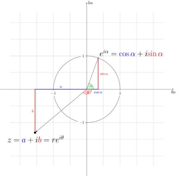
Every complex number \(a+ib\) can be visualized in the complex plane \(\mathbb{C}\). It can be viewed either as the point with the coordinate \((a,b)\) or as a vector starting from \(( 0,0 )\) to the point \((a,b)\).
Also every complex number \(a+ib\) can be represented in the exponential form conveniently by using the Euler’s formula \(e^{i\alpha} = \cos\alpha + i\sin\alpha\). One complex number have unique Cartesian form but many expoential forms. Taking \(1+i\) for example, its expoential form can be \(\sqrt{2}e^{i(\pi/4 + 2n\pi)}, n\in \{ \ldots, -2,-1,0,1,2,\ldots \}\). When we express a complex number in expoential form, it helps to keep a concept of rotation in mind. In the complex plane \(\mathbb{C}\), a complex number will return to itself if it rotates a multiple of \(2\pi\) around the origin point with radius equal to its modulus. please keep the concept of roatation in mind and it will become increasingly important during our later study.
In the development of complex analysis, \(a+ib\) has another form \(r\angle \theta\), where \(r\) is the modulus and \(\theta\) the argument (or the angle). Obviously, this notation is not as good as the expoential form, espacialy when we want to do complex analysis such as differentiation and integration. We just mention it here for the sake of completion. The expoential form will be deployed from now on.
Now, let’s go back to Problem 1.1 and Problem Problem 1.2. It’s easy to figure the answers out using the Euler’s formula. Let’s do more to show them on the complex plane keeping the concept of rotation in mind.
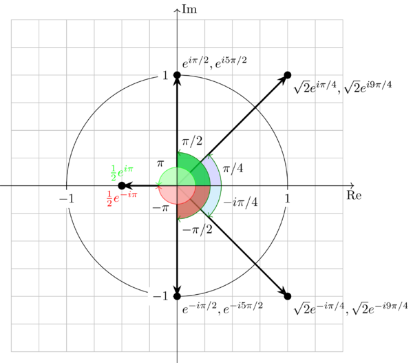
From Figure 1 , taking \(\color{green}{\tfrac{1}{2}e^{i\pi}}\) and \(\color{red}{\tfrac{1}{2}e^{-i\pi}}\) for example, in the complex plane, they are the same point \(-\tfrac{1}{2}\) which means \(-\tfrac{1}{2}\) can be reached by rotating \(\tfrac{1}{2}\) with angle \(\pi\) anti-clockwise or with angle \(-\pi\) clockwise. Essentially, this is because that \(e^{i\theta} = e^{i(\theta + 2n\pi)}, n\in \{\ldots,-2,-1,0,1,2,\ldots\}\). It’s straightforward that \(e^{i\pi} = e^{i(\pi + 2(-1)\pi)} = e^{-i\pi}\).
In the end of Problem 1.1 and Problem 1.2, I want to say more about expressing \(\tfrac{1+i}{1-i}\) in its polar form. There are two methods to get the polar form:
multiply the fraction’s numerator and denominator by \(( 1 + i )\)
So we have:
\begin{eqnarray*} \frac{1+i}{1-i}& = & \frac{(1+i)(1+i)}{(1-i)(1+i)} \\
&=& \frac{2i}{2} = i \end{eqnarray*}express the numerator and denominator in expoential form first, then do the following calculation.
\begin{eqnarray*} \frac{1+i}{1-i} &=& \frac{\sqrt{2}e^{i\pi/4}}{\sqrt{2}e^{-i\pi/4}} \\
&=& e^{i2\pi/4} = e^{i\pi/2} = i \end{eqnarray*}
3 Problem 1.3
Problem 1.3: Determine the values of \(P_{\infty}\) and \(E_{\infty}\) for each of the following signals:
\begin{equation*}
\begin{array}{ll}
\mathrm{(a)} \quad x_{1}(t) = e^{-2t}u(t) & \mathrm{(b)} \quad x_{2}(t) = e^{i(2t + \pi/4)} \\
\mathrm{( c)} \quad x_{3}(t) = \cos(t) & \mathrm{(d)} \quad x_{1}[n] = (\tfrac{1}{2})^{n} u[n] \\
\mathrm{( e )} \quad x_{2}[n] = e^{i(\pi/2n + \pi/8)} & \mathrm{(f)} \quad x_{3}[n] = \cos(\tfrac{\pi}{4}n)
\end{array}
\end{equation*}
Before solving this problem, let’s review the definition of \(P_{\infty}\) and \(E_{\infty}\). For a continuous time signal \(x(t)\), we have
\begin{eqnarray}
\label{eq:2}
E_{\infty}&=& \lim_{T\to \infty} \int_{-T}^{T} |x(t)|^{2}\mathrm{d}t \\
P_{\infty}&=& \lim_{T\to \infty} \frac{1}{2T}\int_{-T}^{T} |x(t)|^{2}\mathrm{d}t = \lim_{T\to\infty} \frac{E_{\infty}}{2T}
\end{eqnarray}
For a discrete time signal \(x[n]\), we have:
\begin{eqnarray}
\label{eq:3}
E_{\infty}&=& \lim_{N\to \infty} \sum_{n=-N}^{+N} |x[n]|^{2} \\
P_{\infty}&=& \lim_{N\to \infty} \frac{1}{2N+1} \sum_{n=-N}^{+N} |x[n]|^{2} = \lim_{N\to\infty} \frac{E_{\infty}}{2N+1}
\end{eqnarray}
Equation (\ref{eq:2})(\ref{eq:3}) are not only mathmatical definitions but also related to physical quantities such as power and energy in a physical system. For an electric circuit, taking the voltage \(v(t)\) and current \(i(t)\) across a resistor for example, the power at time \(t\) can be calculated by:
\begin{equation} \label{eq:4} p(t) = v(t)i(t) = \frac{v^{2}(t)}{R} \end{equation}
Let’s go back to equation (\ref{eq:2}) and equation(\ref{eq:3}), if \(E_{\infty}< \infty\) we say that the signal has finite energy otherwise infinite energy. If \(P_{\infty} <\infty\) we say that the signal has finite power otherwise infinite power.
Next let’s determine the values of \(P_{\infty}\) and \(E_{\infty}\) for the given signals.
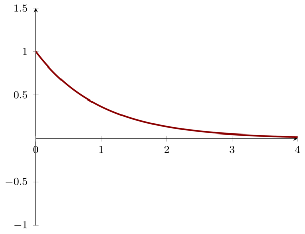
3.1 Problem1.3a \(\mathbf{(a)}: x_{1}(t)= e^{-2t}u(t)\)
\begin{eqnarray*}
E_{\infty} & = & \int_{\infty}^{\infty} |e^{-2t}u(t)|^{2} \mathrm{d}t \\
&=& \int_{0}^{\infty} e^{-4t} \mathrm{d}t \\
&=& \frac{1}{4}
\end{eqnarray*}
So, it’s straightforward that:
\begin{equation} \label{eq:5} P_{\infty} = \lim_{T\to \infty} \frac{E_{\infty}}{2T} = 0 \end{equation}
3.2 Problem1.3b \(\mathbf{(b)}: x_{2}(t)= e^{i(2t+\pi/4)}\)
We have \(|e^{i(2t+\pi/4)}| = 1\) , therefore
\begin{eqnarray*}
E_{\infty}&=& \int_{\infty}^{\infty} |x_{2}(t)= e^{i(2t+\pi/4)}|^{2} \mathrm{d}t \\
&=& \infty
\end{eqnarray*}
For power \(P_{\infty}\), we have:
\begin{eqnarray*}
P_{\infty}&= &\lim_{T\to\infty} \frac{1}{2T}\int_{-T}^{T} |x_{2}(t)|^{2} \mathrm{d}t \\
&=& 1
\end{eqnarray*}
This signal has constant power. If you keep the concept of rotation mentioned in Problem 1, you will notice immediately that all the points generated by \(x_{2}(t)\) lies on the unit circle.
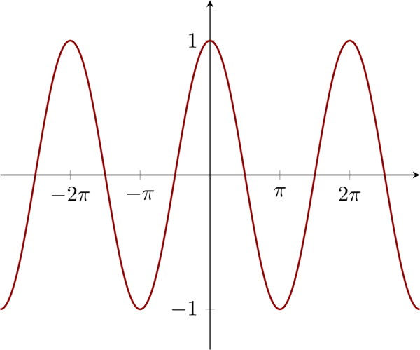
3.3 Problem 1.3c \(\mathbf{( c)}:x_{3}(t)=\cos(t)\)
\begin{eqnarray*}
E_{\infty}&=& \lim_{T\to\infty} \int_{-\infty}^{\infty} |x_{3}(t)|^{2} \mathrm{d}t \\
&=& \int_{\infty}^{\infty} \cos(t)^{2} \mathrm{d}t = \infty
\end{eqnarray*}
\begin{eqnarray*}
P_{\infty}&=& \lim_{T\to\infty} \frac{1}{2T}\int_{-T}^{T} |x_{3}(t)|^{2} \mathrm{d}t \\
&=& \lim_{T\to\infty}\frac{1}{2T} \int_{-T}^{T} \cos(t)^{2} \mathrm{d}t \\
&=& \lim_{T\to\infty} \frac{1}{2T} \int_{-T}^{T} \frac{1+\cos(2t)}{2} \mathrm{d}t = \frac{1}{2}
\end{eqnarray*}
\(x_{3}(t)\) can be visualized as follows:
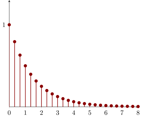
3.4 Problem 1.3d \(\mathbf{(d):} \quad x_{1}[n] = (\tfrac{1}{2})^{n} u[n]\)
By definition, we have:
\begin{eqnarray*}
E_{\infty}&=&\lim_{N\to\infty}\sum_{n=-N}^{N} \big((\tfrac{1}{2})^{n}u[n]\big)^{2} \\
&=&\lim_{N\to\infty}\sum_{n=0}^{N} (\tfrac{1}{4})^{n} \\
&=& \tfrac{4}{3}
\end{eqnarray*}
Then,
\begin{eqnarray*}
P_{\infty}&=& \lim_{N\to\infty} \frac{1}{2N+1} \sum_{n=-N}^{N} \big((\tfrac{1}{2})^{n}u[n]\big)^{2} \\
&=& 0
\end{eqnarray*}
\(x_{1}[n]\) can visualized as:
4 Problem 1.4
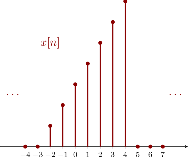
Problem 1.4: Let \(x[n]\) be a signal with \(x[n]=0\) for\(n< -2\) and \(n>4\), for each signal given below, determine the values of \(n\) for which it is guaranteed to be zero.
\begin{eqnarray*}
\mathbf{ (a) } & & x[n-3] \\
\mathbf{ (b) } & & x[n+4] \\
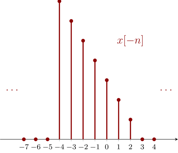
\mathbf{ ( c) } & & x[-n] \\
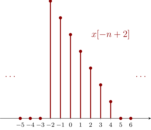
\mathbf{ (d) } & & x[-n+2] \\
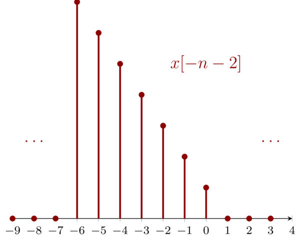
\mathbf{ (e) } & & x[-n-2]
\end{eqnarray*}
For the given signals \(\mathbf{(a)}\) to \(\mathbf{(e)}\), the transformations of the variable \(n\) will change the interval in which the signals are zero. For the convenience of calculation, we write the origin signal as:
\begin{equation*} x[m] = 0, m< -2 \quad \mathrm{and} \quad m>4 \end{equation*}
We can visualize \(x(m)\) as below (I just give an example, you can name any signal that satisfy \(x[m] = 0, m< -2 \ \mathrm{and} \ m>4 \)):
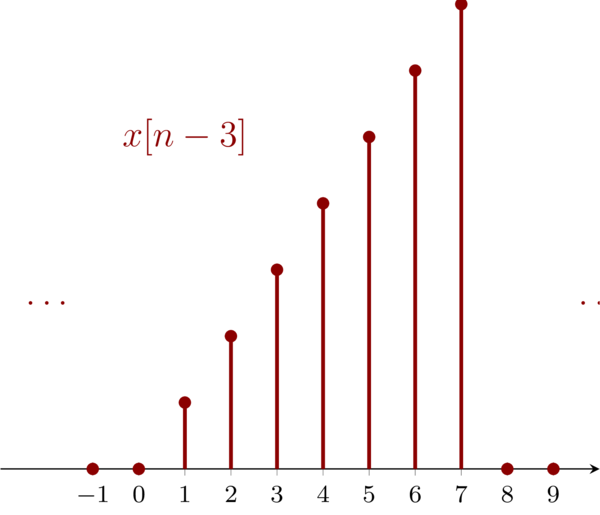
4.1 Problem 1.4a \(\mathbf{(a)}:x[n-3]\)
For signal \(\mathbf{(a)}\), to get the interval where \(x[n-3] = 0 \), we have:
\begin{eqnarray*}
m=n-3 &<& -2 \\
m=n-3 &>& 4
\end{eqnarray*}
Then, we have \( n < 1 \ \mathrm{and} \ n > 7\) from which we can see that the new signal is a right shift three relative to the origin signal, i.e. new signal is delayed with three.
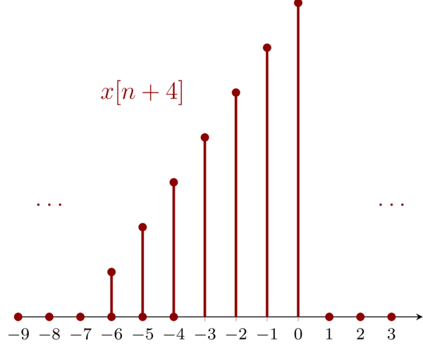
4.2 Problem 1.4b \(\mathbf{(b)}:x[n+4]\)
For signal \(\mathbf{(b)}\), we have:
\begin{eqnarray*}
m=n+4&<&-2 \\
m=n+4&>&4
\end{eqnarray*}
Then, we have \(n<-6\ \mathrm{and}\ n>0\) from which we can see that the new signal is a left shift four relative to the origin signal, i.e. new signal is advanced with four.
4.3 Problem 1.4c \(\mathbf{( c)}: x[-n]\)
For signal \(\mathbf{( c )}\), we have:
\begin{eqnarray*}
m=-n&<&-2 \\
m=-n&>&4
\end{eqnarray*}
Then, we have \(n>2\ \mathrm{and} \ n<-4\) from which we can see that the new signal is a reversal of the origin signal.
4.4 Problem 1.4d \(\mathbf{(d)}: x[-n+2]\)
for signal \(\mathbf{(d)}\), we have:
\begin{eqnarray*}
m=-n+2&<&-2 \\
m=-n+2&>&4
\end{eqnarray*}
Then, we have \(n>4\ \mathrm{and}\ n<-2\). For \(x[-n+2]\), we can first flip the original signal then right shift the flipped signal by 2. Notice the contents in the brackets \(-(n+2)\). I would like treat it as \(-(n-2)\), by which I know that the minus symbol means reversal and \(-2\) means right shift by 2.
4.5 Problem 1.4e \(\mathbf{(e)}: x[-n-2]\)
For signal \(\mathbf{(e)}\), we have:
\begin{eqnarray*}
m=-n-2&<&-2 \\
m=-n-2&>&4
\end{eqnarray*}
Then, we have \( n>0 \ \mathrm{and}\ n<-6 \). To get the new signal, we have to filp the original signal first then left shift the flipped signal by two.
5 Problem 1.5
Let \(x(t)\) be a signal with \(x(t)=0, \ x<3\). For each signal given below, determine the values of \(t\) for which it is guaranteed to be zero.
\begin{equation*}
\begin{array}{ll}
\mathbf{(a)}: x(1-t) \qquad & \mathbf{(b)}: x(1-t) + x(2-t)\qquad \\
\mathbf{( c)}: x(1-t)x(2-t)\qquad & \mathbf{(d)}: x(3t) \qquad \\
\mathbf{(e)}: x(t/3)\qquad & \\
\end{array}
\end{equation*}
For signal \(\mathbf{(a)}: x(1-t) \), we have:
\begin{equation*} 1-t < 3 \end{equation*}
So, \(t>-2\). Signal \(\mathbf{(a)}: x(1-t) \) can be achieved by flipping the origin signal first then right shifting one.
For signal \(\mathbf{(b)}: x(1-t) + x(2-t) \) , we have:
\begin{eqnarray*}
1-t&< &3 \\
2-t&<& 3
\end{eqnarray*}
Because it a “\(+\)” between \(x(1-t)\) and \(x(2-t)\) so only when both of the two signals are zero, the result will be zero. For the first part we have the value zero when \(t>-2\) the second \(t>-1\), so the result will be the intersect of these two intervals, i.e. \(t>-1\) . we achieve signal \(\mathbf{(b)}: x(1-t) + x(2-t) \) by adding signal \(\mathbf{(a)}: x(1-t) \) with a second signal \(x(2-t)\) which can be achieved by flipping it first then right shifting two.
For signal \(\mathbf{( c)}: x(1-t)x(2-t) \), \(x(1-t)\) is multiplied by \(x(2-t)\), so if any one of these two signals is zero, the result is zero. Based on the result of signal \(\mathbf{( b )}\), we have \(t>-2\).
For signal \(\mathbf{( d )}: x(3t)\), we have:
\begin{equation*} 3t < 3 \end{equation*}
Then, \(t<1\). The signal is compressed by \(3\).
For signal \(\mathbf{( e )}: x(t/3)\), we have:
\begin{equation*} t/3 < 3 \end{equation*}
Then, \(t<9\). The signal is streched by \(3\).
6 Problem 1.6
Determine whether or not each of the following signals is periodic:
\begin{eqnarray*}
&& \mathbf{(a)}: x_{1}(t) = 2e^{i(t+\pi/4)}u(t) \\
&& \mathbf{( b )}: x_{2}[n] = u[n] + u[-n] \\
&& \mathbf{( c)}: x_{3}[n] = \sum_{k=-\infty}^{\infty} \{ \delta[n-4k] - \delta[n-1-4k] \}
\end{eqnarray*}
- \(x_{1}(t)\) is not periodic because \(u(t) = 0, t<0\)
\(x_{2}[n]\) is not periodic because
\begin{equation*} x_{2}[n] = \begin{cases} 2 & n=0 \\
1 & n\neq 0 \end{cases} \end{equation*}For signal \(x_{3}[n]\) we know that with a \(n\), \(\delta[n-4k]\) and \(\delta[n-1-4k]\) can not be zero at the same time. Because \(k\) and \(n-4k\) must be integers, \(\delta[n-4k]\) and \(\delta[n-1-4k]\) will repeat themself every four steps. Furthermore, for every \(n\), the \(k\) runs from \(-\infty \) to \(\infty\), and only one \(k\) will match the \(n\) to set \(\delta[n-4k]\) or \(\delta[n-1-4k]\) as zero. We can test it by setting \(n = 0,1,2,\ldots\)
\begin{eqnarray*} && x[0] = 1,\quad x[1] = -1, \quad x[2] = 0, \quad x[3] = 0 \\
&& x[4] = 1,\quad x[5] = -1, \quad x[6] = 0, \quad x[7] = 0 \\
&& x[8] = 1,\quad x[9] = -1, \quad x[10] = 0, \quad x[11] = 0 \end{eqnarray*}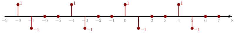
7 Problem 1.7
For each signal given below, determine all the values of the independent variable at which the even part of the signal is guaranteed to be zero.
\begin{equation*}
\small
\begin{array}{ll}
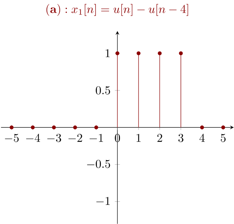
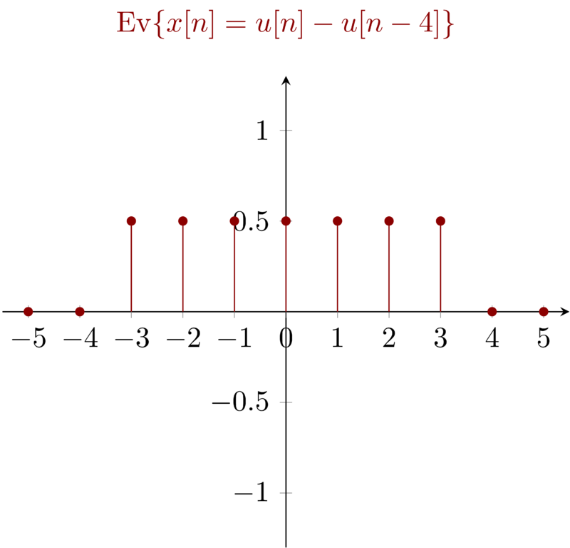
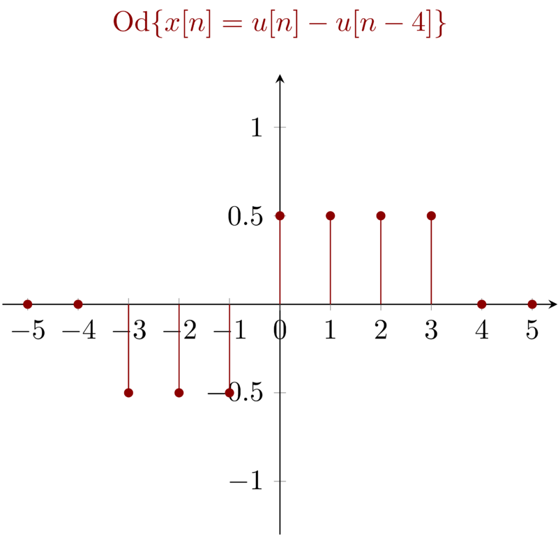
\mathbf{(a)}: x_{1}[n] = u[n] - u[n-4] \qquad & \mathbf{(b)}: x_{2}(t) = \sin(\tfrac{1}{2} t) \qquad \\
\mathbf{( c)}: x_{3}[n] = (\frac{1}{2})^{n} u[n-3] \qquad & \mathbf{(d)}: x_{4}(t) = e^{-5t}u(t+2) \\
\end{array}
\end{equation*}
7.1 Problem 1.7a \(\mathbf{(a)}: x_{1}[n] = u[n] - u[n-4] \)
Any signal \(x_{1}(t)\) consists of two parts, even part \(\mathrm{Ev} \{x_{1}(t)\} \) and odd part \( \mathrm{Od} \{ x_{1}(t)\} \). For signal \( \mathbf{(a)} \), when the signal is zero, we have the domain of the independent value \( n< 0 \) and \( n \geq 4 \) , so the even part of the signal will be zero when \( n\leq 4 \) and \(n\geq 4\). \(x_{t}(t)\) and its even part and odd part can be illustrated as:
7.2 Problem 1.7b \(\mathbf{(b)}: x_{2}(t) = \sin(\tfrac{1}{2} t) \)
For signal \(x_{2}(t) = \sin (\frac{1}{2} t)\), because it is an odd signal, so for all \(t\), the even part of \(x_{2}(t)\) is zero.
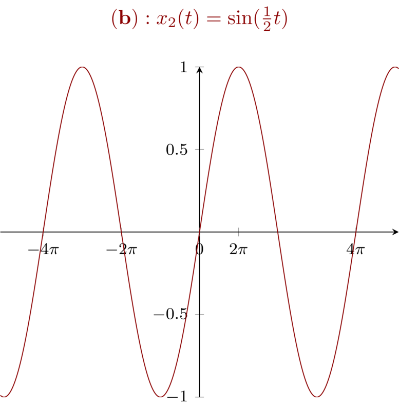
Notice that for \(\sin(\frac{1}{2}t)\), the signal can be obtained by streching \(\sin(t)\) with a factor \(2\). In particular, the fundamental period is \(4\pi\).
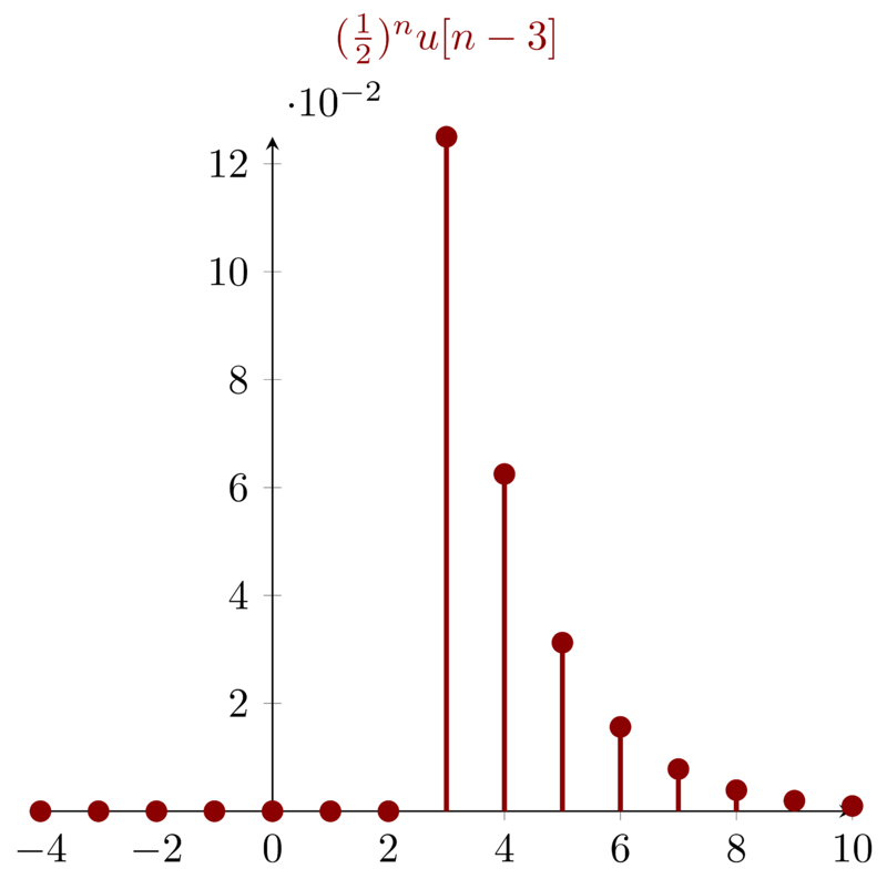
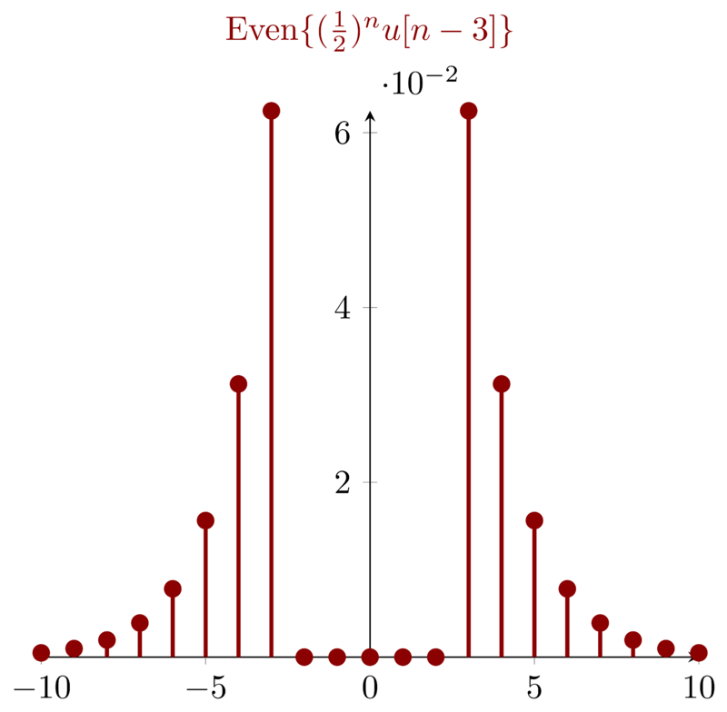
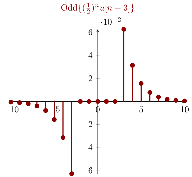
7.3 Problem 1.7c \(\mathbf{( c)}: x_{3}[n] = ( \frac{1}{2} )^{n} u[n-3] \)
For signal \(x_{3}[n] = ( \frac{1}{2} )^{n} u[n-3] \), which will be zeros for \(n<3\). By definition, the even part of \(x_{3}[n]\) will be zeros for \(|n| < 3\). Actually, we do not visualize the signal to draw such a conclusion. For the sake of visualization, I illustrate the signal as below:
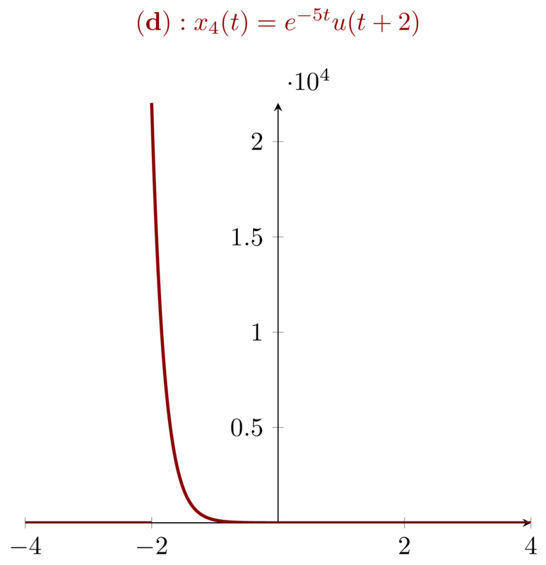
7.4 Problem 1.7d \(\mathbf{(d)}: x_{4}(t) = e^{-5t}u(t+2) \)
For signal \(\mathbf{(d)}: x_{4}(t) = e^{-5t}u(t+2) \), we have \(x_{4}(t) = 0,
t<-2\). Because the even and odd part is symmetrical with y-axis, there is no
\(t\) at which the even and odd part of will be zero.
8 Problem 1.8
Express the real part of each of the following signals in the form \(Ae^{-at}\cos(\omega t + \phi)\), where \(A,a,\omega, \phi\) are real numbers with \(A>0\) and \(-\pi < \phi \leq \pi \):
\begin{equation*}
\small
\begin{array}{ll}
\mathbf{( a )}: x_{1}(t) = -2 & \mathbf{( b )}: x_{2}(t) = \sqrt{2}e^{i\pi/4}\cos(3t + 2\pi) \\
\mathbf{( c )}: x_{3}(t) = e^{-t}\sin(3t + \pi) & \mathbf{( d )}: x_{4}(t) = i e^{(-2+i100)t}
\end{array}
\end{equation*}
- \(\mathrm{Re}\{x_{1}(t)\} = -2 = 2e^{-0t}\cos(0t + \pi) \) with \(A = 2, a=0, \omega = 0, \phi = \pi\)
- \( \mathrm{Re} \{x_{2}(t)\} = \mathrm{Re} \{ \sqrt{2} ( \cos( \pi/4 ) + i \sin (\pi/4) ) \cos(3t) \} = \cos(3t) = e^{-0t}\cos( 3t + 0 ) \) with \(A = 1\), \( a = 0 \), \( \omega = 3 \),\(\phi = 0\)
- \( \mathrm{Re} \{ x_{3}(t) \} = \mathrm{Re} \{ e^{-t} \sin ( 3t + \pi ) \} = e^{-t}\cos(3t + \pi/2) \) with \(A=1\), \(a=1\), \(\omega=3\), \(\phi=\pi/2\)
- \( \mathrm{Re} \{x_{4}(t)\} = \mathrm{Re} \{ e^{i\pi/2} e^{(-2+i100)t} \} = \mathrm{Re}\{ e^{(-2 + i100)t + i\pi/2} \} = e^{-2t}\cos(100t + \pi/2) \) with\(A = 1\), \(a=2\), \(\omega=100\), \(\phi=\pi/2\)
9 Problem 1.9
Determine whether or not each of the following signals is periodic. If a signal is periodic, specify its fundamental period.
\begin{equation*}
\begin{array}{ll}
\mathbf{( a )}: x_{1}(t) = ie^{i10t} & \mathbf{( b )}: x_{2}(t) = e^{(-1 + i)t} \\
\mathbf{( c )}: x_{3}[n] = e^{i7\pi n} & \mathbf{( d )}: x_{4}[n] = 3e^{i( 3\pi ( n + 0.5 ) ) / 5} \\
\mathbf{( e )}: x_{5}[n] = 3e^{ i3/5(n+ 0.5 )} &
\end{array}
\end{equation*}
During figuring all the problems, we have to keep in mind that for a complex number after rotating \(2\pi \) around the origin the number returns to itself.
- For \(x_{1}(t)\), only when phase \(10t\) increases multiples of \(2\pi\), does the signal return to itself. So the fundamental period is \( \frac{2\pi}{10} = \frac{\pi}{5} \).
- For \(x_{2}(t)\), which can be expressed as \(e^{-t}e^{it}\), because the factor \(e^{-t}\) , the signal is not periodic.
- For \(x_{3}[ n ]\), we have \(e^{i7\pi n} = e^{i\pi n}\), then the fundamental period is \(\frac{2\pi}{\pi} = 2\)
For \(x_{4}[n]\), we have:
\begin{equation*} \frac{3\pi N}{5} = 2\pi m \end{equation*}
Then \(N = \frac{10m}{3}\), So fundamental period \(N=10\) when \(m=3\).
For \(x_{5}[n]\), because \( m\frac{2\pi \times 5}{ 3 } \) is an irrational number, so the signal is not periodic.
10 Problem 1.10
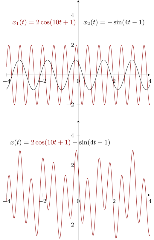
Determine the fundamental period of the signal \(x(t) = 2\cos(10t + 1) - \sin(4t -1)\)
\(x(t)\) consists of two parts, \(2\cos(10t + 1)\) and \(-\sin(4t -1)\). First, We figure out the fundamental period for these two signals respectively. For \(cos(10t + 1)\), \(10T_{1} = 2\pi \to T_{1} = \frac{\pi}{5}\); For \(-\sin(4t -1)\) , we have \( 4T_{2} = 2\pi \to T_{2} = \frac{\pi}{2} \) . Then, the fundamental period \(T = mT_{1} = nT_{2}\) ,So when \(m=5\) and \(n=2\) , we have \(T=\pi\) , \(T\) is the least common multiples of \(T_{1}\) and \(T_{2}\)
11 Problem 1.11
Determine the fundamental period of the signal \(x[n] = 1 + e^{i4\pi n/7} - e^{i2\pi n/5}\)
\(x[n]\) consists of two main parts, \( e^{i4\pi n/7} \) and \(e^{i2\pi n/5}\). We have to figure out the two fundamental periods respectively then calculate the least common multiple of the two fundamental periods.
For the first part we have:
\begin{equation*} N_{1} = m \frac{2\pi}{ 4\pi /7 } = m\frac{7}{2} \end{equation*}
So when \(m=2\), we have \(N_{1} = 7\).
For the second part we have:
\begin{equation*} N_{2} = m \frac{2\pi}{ 2\pi /5 } \end{equation*}
So when \(m=1\), we have \(N_{2} = 5\). The lease common multiple of \(N_{1}\) and \(N_{2}\) is 35, i.e. the fundamental period of \(x[n]\)
It is easy to validate it. We have \(x[0] = 1 = x[35]\)
12 Problem 1.12
Consider the discrete-time signal
\begin{equation*} x[n] = 1- \sum_{k=3}^{\infty}\delta[n-1-k] \end{equation*}
Determine the values of the integers \(M\) and \(n_{0}\) so that \(x[n]\) may be expressed as
\begin{equation*} x[n] = u[Mn - n_{0}] \end{equation*}
By definition of \(\delta[n]\) , we know that when \(n=1+k\), \(\delta[n-1-k] = 1\). For \(x[n]\), because \(k\geq 3\), so for every \(n\geq 4\), there will always be one \(k\) such that \(x[n] = 0\). However, for every \(n\leq 3\), such that \(\sum_{k=3}^{\infty} \delta[n-1-k] = 1 \), i.e. \(\sum_{k=3}^{\infty} \delta[n-1-k] = 0 \) for all \(n\leq 3\) , So \(x[n] = 1\) for all \(n\leq 3\).
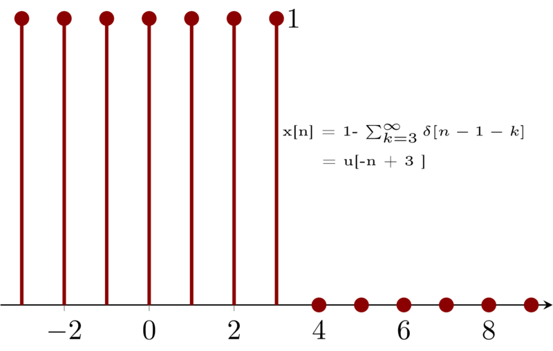
Then, by the definition of unit step function, we have \(M=-1\) and \(n_{0}= -3\) . We can see that \(x[n]\) can be obtained by flipping the unit step signal then right shifting it with \(3\).
13 Problem 1.13
Consider the continuous-time signal
\begin{equation*} x(t) = \delta(t+2) - \delta(t-2) \end{equation*}
Calculate the value of \(E_{\infty}\) for the signal
\begin{equation*} y(t) = \int_{-\infty}^{t} x(\tau) \mathrm{d} \tau \end{equation*}
First let’s visualize \(x(t)\) which can be shown as below
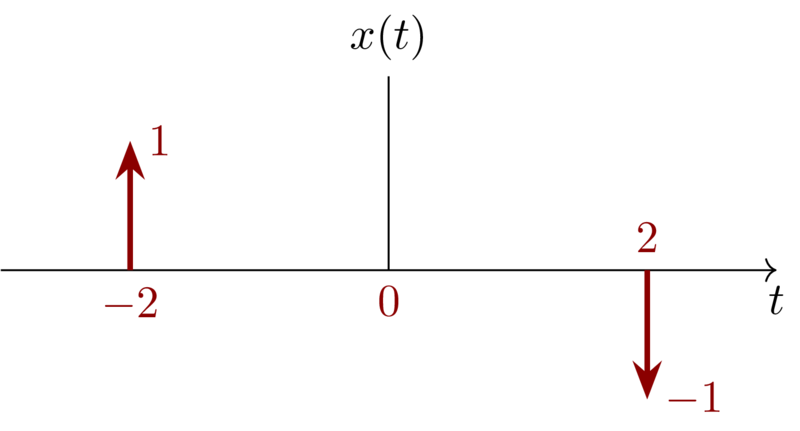
Notice the “\(1\)” along with the end of the impulses at \((-2,0)\) and \((2,0)\) only represent that the area of the impulse is \(1\).
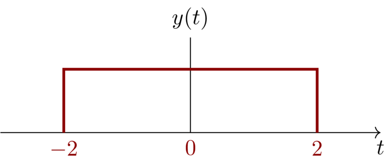
For \(y(t)\), we have:
\begin{eqnarray*}
y(t)&=& \int_{-\infty}^{t} x(\tau) \mathrm{d} \tau\\
&=&
\begin{cases}
0 & t < -2 \\
1 & -2 \leq t < 2 \\
0 & 2 \leq t
\end{cases}
\end{eqnarray*}
Then,
\begin{equation*} E_{\infty} = \lim_{T\to\infty} \int_{-T}^{T} |y(t)|^{2} \mathrm{d}t = 4 \end{equation*}
14 Problem 1.14
- CLOSING NOTE
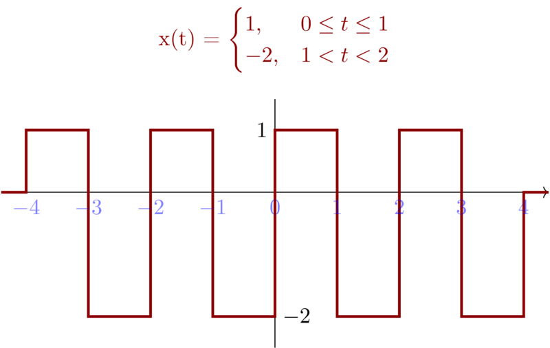
Consider a periodic signal
\begin{equation*}
x(t) =
\begin{cases}
1, & 0\leq t\leq 1 \\
-2, & 1 < t <2
\end{cases}
\end{equation*}
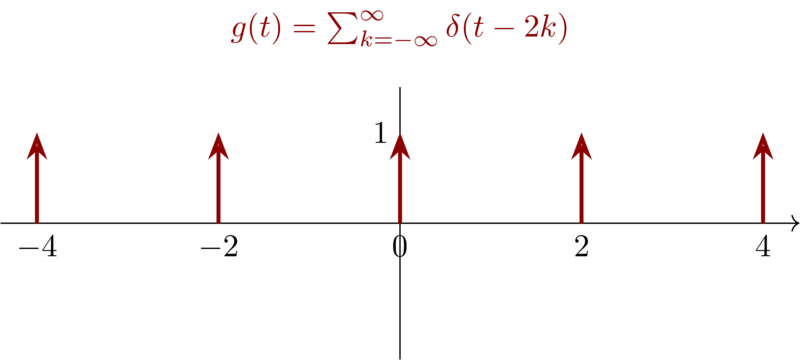
with period \(T=2\), The derivative of this signal is related to the “impulse train”
\begin{equation*} g(t) = \sum_{k=-\infty}^{\infty} \delta(t-2k) \end{equation*}
with period \(T=2\). It can be shown that
\begin{equation*} \frac{\mathrm{d}x(t)}{\mathrm{d}t} = A_{1}g(t-t_{1}) + A_{2} g(t-t_{2}) \end{equation*}
Determine the values of \(A_{1},t_{1},A_{2}\) and \(t_{2}\)
First let’s visualize \(x(t)\) and \(g(t)\) :
Then we try to figure out \(\frac{\mathrm{d}x(t)}{\mathrm{d}t}\) . By definition of \(\delta (t)\) in section of the textbook, we know that,
\begin{equation*} \frac{\mathrm{d}x(t)}{\mathrm{d}t} = 3\sum_{k=-\infty}^{\infty} \sigma(t-2k ) -3 \sum_{k=-\infty}^{\infty} \sigma(t-2k -1) \end{equation*}
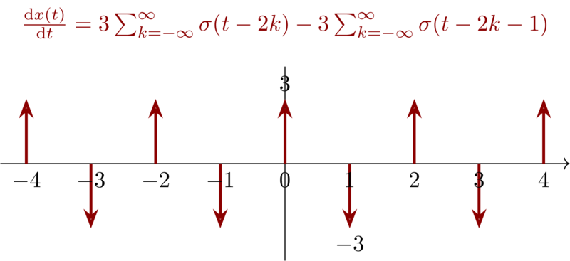
Compared the result with \(g(t)\), then we have \(A_{1} = 3\), \(A_{2} = -3\), \(t_{1} = 0\) ,\(t_{2} = 1\)
15 Problem 1.15
Consider a system \(S\) with input \(x[n]\) and output \(y[n]\). This system is obtained through a series interconnection of a system \(S_{1}\) followed by a system \(S_{2}\). The input-output relationships for \(S_{1}\) and \(S_{2}\) are:
\begin{eqnarray*}
S_{1}:\quad y_{1}[n]&=& 2x_{1}[n] + 4x_{1}[n-1] \\
S_{2}:\quad y_{2}[n]&=& x_{2}[n-2] + \frac{1}{2}x_{2}[n-3]
\end{eqnarray*}
where \(x_{1}[n]\) and \(x_{2}[n]\) denote input signals.
- Determine the input-output relationship for system \(S\)
- Does the input-output relationship of system \(S\) change if the order in which \(S_{1}\) and \(S_{2}\) are connected in series is reversed (i.e., if \(S_{2}\) follows \(S_{1}\))?
15.1 \(S_{1}\) is followed by \(S_{2}\)
Because \(S_{1}\) is followed by \(S_{2}\), then the output of \(S_{1}\) is the input of \(S_{2}\) i.e., \(y_{1}[n]\) can be treated as \(x_{2}[n]\) , So,
\begin{eqnarray*}
y_{2}[n]&=& x_{2}[n-2] + \frac{1}{2}x_{2}[n-3] \\
&=& \underbrace{2x_{1}[n-2] + 4x_{1}[n-2-1]}_{y_{1}[n-2]} + \underbrace{\tfrac{1}{2} \Big( 2x_{1}[n-3] + 4x_{1}[n-3-1] \Big)}_{\frac{1}{2}y_{1}[n-3]} \\
&=& 2x_{1}[n-2] + 5x_{1}[n-3] + 2x_{1}[n-4]
\end{eqnarray*}
\(y_{2}\) is the final output of system \(S\), and \(x_{1}[n]\) the input.
15.2 \(S_{2}\) is followed by \(S_{1}\)
If \(S_{2}\) is followed by \(S_{1}\), then \(y_{2}[n]\) can be treated by \(x_{1}[n]\), \(y_{1}[n]\) is the final output of system \(S\) and \(x_{2}[n]\) the input.
\begin{eqnarray*}
y_{1}[n]&=& 2x_{1}[n] + 4x_{1}[n-1] \\
&=& \underbrace{2 \Big( x_{2}[n-2] + \tfrac{1}{2} x_{2}[n-3] \Big)}_{2{y_{2}[n]}} + \underbrace{4 \Big( x_{2}[n-1-2] + \tfrac{1}{2}x_{2}[n-3-1] \Big)}_{4y_{2}[n]} \\
&=& 2x_{2}[n-2] + 5x_{2}[n-3] + 2x_{2}[n-4]
\end{eqnarray*}
After comparing the result from (1) we can see that the two systems are identical, no matter who ( either \(S_{1}\) or \(S_{2}\)) comes first.
Later we will learn that for any number of linear systems, the input-output relationship does not change no matter what order by which they are concatenated.
16 Problem 1.16
Consider a discrete-time system with input \(x[n]\) and output \(y[n]\). The input-output relationship for this system is
\begin{equation*} y[n] = x[n]x[n-2] \end{equation*}
- Is the system memoryless?
- Determine the output of the system when the input is \(A\delta[n]\), where \(A\) is any real or complex number.
- Is the system invertible?
Is the system memoryless?
By definition, a system is memoryless if its output for each value of the independent variable at a given time is dependent on the input at only the same time. Obviously, the output \(y[n]\) is dependent on not only the current time \(x[n]\) but also \(x[n-2]\). So the system is not memoryless.
The output of the system \(y[n] = x[n]x[n-2] = A \delta[n] A \delta[n-2] = A^{2} \delta[n]\delta[n-2]\). By the definition of \(\delta[n]\), we have \(y[n] = 0\)
Is the system invertible?
A system is said to be invertible if distinct inputs lead to distinct outputs. We can take it as the input and output has one-to-one map. For the given system, if we get one positive value, we cannot determine where the sign come from. i.e. it can be have a positive \(x[n]\) and a positive \(x[n-2]\) or a negative \(x[n]\) and a negative \(x[n-2]\). So the system is not invertible.
17 Problem 1.17
Consider a continuout-time system with input \(x(t)\) and output \(y(t)\) related by \(y(t) = x( \sin(t) )\).
- Is this system causal?
- Is this system linear?
A system is causal if the output at any time depends on values of the input at only the present and past times. We can anticipate the output of one causal system based on the history of the input. When it comes to \(y(t) = x(\sin(t))\) , we can have \(y(-\pi) = x(0), t=-\pi\). i.e. \(y(-\pi)\) is determined by an input from the future. So the system is not causual.
If a system is linear, we have:
- The response to \(x_{1}(t) + x_{2}(t)\) is \(y_{1}(t) + y_{2}(t)\).
- The response to \(ax_{1}(t) \) is \(ay_{1}(t)\), where \(a\) is any complex constant.
When the input is \(a_{1}x_{1}(\sin(t)) + a_{2}x_{2}(\sin(t)) \), the output will be \(a_{1}y_{1}(t) + a_{2}y_{2}(t)\) . The system is linear.
18 Problem 1.18
Consider a discrete-time system with input \(x[n]\) and output \(y[n]\) related by
\begin{equation*} y[n] = \sum_{k=n-n_{0}}^{n+n_{0}} x[k] \end{equation*}
where \(n_{0}\) is a finite positive integer.
- Is this system linear?
- Is this system time-invariant?
- If \(x[n]\) is known to be bounded by a finite integer \(B\) , (i.e. \(|x[n]| < B\) for all \(n\)), it can be shown that \(y[n]\) is bounded by a finite number \(C\). We conclude that the given system is stable. Express \(C\) in terms of \(B\) and \(n_{0}\).
18.1 linearity
According to definition of linearity, suppose we have two inputs \(x_{1}[n]\) and \(x_{2}[n]\), the reponse is \(y_{1}[n]\) and \(y_{2}[n]\). i.e.
\begin{eqnarray*}
y_{1}[n]&=& \sum_{k=n-n_{0}}^{n+n_{0}} x_{1}[k] \\
y_{2}[n]&=& \sum_{k=n-n_{0}}^{n+n_{0}} x_{2}[k] \\
\end{eqnarray*}
Then for \(x_{3}[n] = x_{1}[n] + x_{2}[n]\), we have
\begin{eqnarray*}
y_{3}[n]&=& \sum_{k=n-n_{0}}^{n+n_{0}} x_{3}[k] \\
&=& \sum_{k=n-n_{0}}^{n+n_{0}} (x_{1}[k] + x_{2}[k]) \\
&=&\sum_{k=n-n_{0}}^{n+n_{0}} x_{1}[k] + \sum_{k=n-n_{0}}^{n+n_{0}} x_{2}[k] \\
&=& y_{1}[n] + y_{2}[n]
\end{eqnarray*}
When \(x_{3}[n] = ax_{1}[n]\),
\begin{eqnarray*}
y_{3}[n] &=& \sum_{k=n-n_{0}}^{n+n_{0}} x_{3}[k] \\
&=& \sum_{k=n-n_{0}}^{n+n_{0}} ax_{1}[k] \\
&=& a y_{1}[n]
\end{eqnarray*}
So that the system is linear.
18.2 time invariant
If a system is time invariant, the output does not change if you input the same signal at any time. No matter when you repeat the same experiment, you will get the same output.
For an input \(x_{1}[n]\), we have
\begin{equation*} y_{1}[n] = \sum_{k=n-n_{0}}^{n+n_{0}} x_{1}[k] \end{equation*}
Suppose we have another input \(x_{2}[n] = x_{1}[n-n_{1}]\), so
\begin{eqnarray*}
y_{2}[n]&=& \sum_{k=n-n_{0}}^{n+n_{0}} x_{2}[k] \\
&=& \sum_{k=n-n_{0}}^{n+n_{0}} x_{1}[k-n_{1}] \\
&=& \sum_{k=n-n_{1}-n_{0}}^{n-n_{1}+n_{0}} x_{1}[k] \\
&=& y_{1}[n-n_{1}]
\end{eqnarray*}
So when we have \(x_{2}[n] = x_{1}[n- n_{1}]\), then we have \(y_{2}[n] = y_{1}[n- n_{1}]\). So, the system is time invariant.
18.3 find \(C\)
we know that \(x[n] \leq B\), then
\begin{eqnarray*}
y[n] &=& \sum_{k=n-n_{0}}^{n+n_{0}} x[k] \\
&\leq & \sum_{k=n-n_{0}}^{n+n_{0}} B \\
&=& ( 2n_{0} + 1 ) B
\end{eqnarray*}
So we have \(C \leq ( 2n_{0} +1 )B\).
19 Problem 1.19
For each of the following input-output relationships, determine whether the corresponding system is linear, time invariant or both
\begin{eqnarray*}
\mathbf{(a)}\quad y(t)&=& t^{2} x(t-1) \\
\mathbf{(b)}\quad y[n]&=& x^{2}[n-2] \\
\mathbf{( c)}\quad y[n]&=& x[n+1] - x[n-1] \\
\mathbf{(d)}\quad y( t )&=& \mathrm{Odd}\{ x(t) \}
\end{eqnarray*}
19.1 Problem 1.19a \(\mathbf{(a)}: y(t)= t^{2} x(t-1) \)
Suppose that \(y_{1}(t)\) and \(y_{2}(t)\) are the responses for input \(x_{1}(t)\) and \(x_{2}(t)\), respectively. Given \(x_{3}(t) = ax_{1}(t) + bx_{2}(t)\), then we have:
\begin{equation*} y_{3}(t) = t^{2}x_{3}(t-1) = t^{2} \Big( ax_{1}(t-1) + bx_{2}(t-1) \Big) = ay_{1}(t) + by_{2}(t) \end{equation*}
So the system is linear.
To check whether this system is time invariant, we must determine whether the time-invariant property holds for any input and any time shift \(t_{0}\). Suppose when \(x_{1}(t)\) is applied we have output \(y_{1}(t) = t^{2}x_{1}(t-1)\). We shfit \(x_{1}(t)\) with \(t_{0}\) to get \(x_{2}(t-t_{0})\) and apply it to the system. Then we have \(y_{2}(t) = t^{2}x_{2}(t-t_{0}-1)\) which is not the shifted version of \(y_{1}(t)\) which is \(y_{1}(t-t_{0}) = (t-t_{0})^{2} x_{2}(t-t_{0}-1) \). So the system is not time invariant.
19.2 Problem 1.19b \(\mathbf{(b)}: y[n]= x^{2}[n-2] \)
To check whether the system is linear or not, suppose \(x_{3}[n] = ax_{1}[n] + bx_{2}[n]\) then
\begin{eqnarray*}
y_{3}[n] &=& x_{3}^{2}[n-2] \\
&=& ( ax_{1}[n-2] + bx_{2}[n-2] )^{2} \\
&=& a^{2} x_{1}^{2}[n-2] + b^{2}x_{2}^{2}[n-2] + 2abx_{1}[n-2]x_{2}[n-2] \\
&\neq& ay_{1}[n] + by_{2}[n]
\end{eqnarray*}
So the system is not linear
\(x_{1}[n]\) will generate output \(y_{1}[n] = x_{1}^{2}[n-2]\). Suppose \(x_{2}[n] = x_{1}[n-n_{0}]\), then we have \(y_{2}[n] = x_{2}^{2}[n-2] = x_{1}^{2}[n-n_{0}-2] = y_{1}[n-n_{0}]\) , i.e. when the input shift with \(n_{0}\) the output will all shift with \(n_{0}\). So this system is time invariant
19.3 Problem 1.19c \( \mathbf{( c)}: y[n]= x[n+1] - x[n-1] \)
First, we check whether or not the system is linear. consider
\begin{eqnarray*}
x_{1}[n]&\to& y_{1}[n] \\
x_{2}[n]&\to& y_{2}[n]
\end{eqnarray*}
Let \(x_{3}[n] = ax_{1}[n] + bx_{2}[n]\), then
\begin{eqnarray*}
y_{3}[n]&=& x_{3}[n+1] - x_{3}[n-1] \\
&=& ax_{1}[n+1] + bx_{2}[n+1] - ( ax_{1}[n-1] + bx_{2}[n-1] ) \\
&=& a(x_{1}[n+1] - ax_{1}[n-1]) + b(x_{2}[n+1] - x_{2}[n-2]) \\
&=& a y_{1}[n] + by_{2}[n]
\end{eqnarray*}
So
\begin{equation*} ax_{1}[n] + bx_{2}[n] \to ay_{1}[n] + by_{2}[n] \end{equation*}
The system is linear.
Second, we check whether or not the system is time invariant. let \(x_{2}[n] = x_{1}[n-n_{0}]\) then we have
\begin{equation*} y_{2}[n] = x_{2}[n+1] - x_{2}[n-1] = x_{1}[n-n_{0} + 1] - x_{1}[n-n_{0} -1] = y_{1}[n-n_{0}] \end{equation*}
So the system’s output and input see the same time shift. The system is time invariant
19.4 Problem 1.19d \( \mathbf{(d)}: y(t)= \mathrm{Odd}\{ x(t) \}\)
First, we check whether or not the system is linear. Considering two inputs \(x_{1}(t)\) and \(x_{2}(t)\), we have:
\begin{eqnarray*}
y_{1}(t)&=& \mathrm{Odd}\{ x_{1}(t) \} \\
y_{2}(t) &=& \mathrm{Odd} \{ x_{2}(t) \}
\end{eqnarray*}
Let \(x_{3}(t) = ax_{1}(t) + bx_{2}(t)\), then
\begin{eqnarray*}
y_{3}(t)&=& \mathrm{Odd} \{ x_{3}(t) \} \\
&=& \mathrm{Odd} \{ ax_{1}(t) + bx_{2}(t) \} \\
&=& \mathrm{Odd} \{ax_{1}(t) \} + \mathrm{Odd} \{ bx_{2}(t) \} \\
&=& ay_{1}(t) + by_{2}(t)
\end{eqnarray*}
The system is linear.
Second we check whether or not the system is time-invariant. A system is time invariant if a time shift in the input signal results in an identical shift in the output signal.
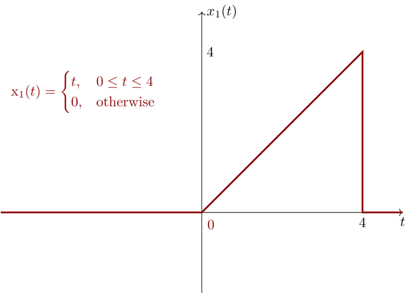
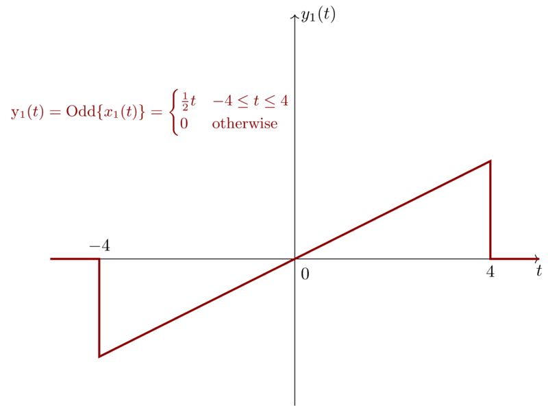
If we shift the input \(x(t)\) and get \(x(t-t_{0})\) then the result \(y(t)\) we become as \(y(t-t_{0})\). Before we check the property of time-invarant, let’s first check one example. Suppose
\begin{equation*}
x_{1}(t) =
\begin{cases}
t, & 0\leq t \leq 4 \\
0, & \mathrm{otherwise}
\end{cases}
\end{equation*}
Then
\begin{equation*}
y_{1}(t) = \mathrm{Odd}\{x_{1}(t)\} = \frac{x_{1}(t)-x_{1}(-t)}{2} =
\begin{cases}
\frac{1}{2}t & -4 \leq t \leq 4 \\
0 & \mathrm{otherwise}
\end{cases}
\end{equation*}
We can visualize \(x_{1}(t)\) and \(y_{1}(t)\) as follows:
If we shift \(x_{1}(t)\) by \(2\) to obtain \(x_{2}(t) = x_{1}(t-2)\), then we have
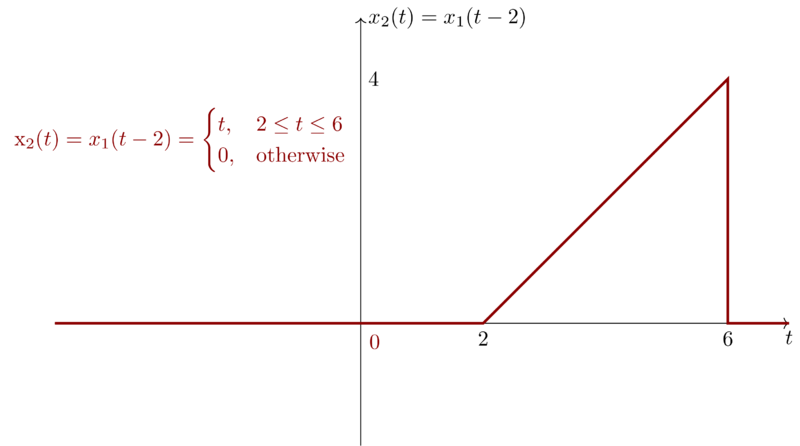
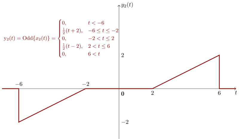
Then we have \(y_{2}(t)\),
\begin{equation*}
y_{2}(t) =
\begin{cases}
0, & t < -6 \\
\tfrac{1}{2}( t+2 ), & -6 \leq t \leq -2 \\
0, & -2 < t \leq 2 \\
\frac{1}{2} (t-2), & 2 < t \leq 6 \\
0, & 6 < t
\end{cases}
\end{equation*}
Then, we visualize \( y_{2}(t) \),
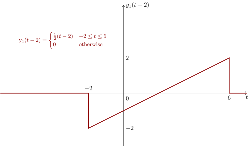
Notice, by shifting \(y_{1}(t)\) by \(2\) , we have \(y_{1}(t-2)\)
\begin{equation*}
y_{1}(t-2) =
\begin{cases}
\frac{1}{2} (t-2) & -2 \leq t \leq 6 \\
0 & \mathrm{otherwise}
\end{cases}
\end{equation*}
Now, we can derive that \(y_{1}(t-2) \neq y_{2}(t)\) . Hence, The system is not time invariant .
Also we can visualize \(y_{1}(t-2)\) to see how different \(y_{1}(t-2)\) and \(y_{2}(t)\) are.
Now, we deduce that the system is time-invariant. For \(x_{1}(t)\), we have,
\begin{equation*} y_{1}(t) = \mathrm{Odd}\{ x_{1}(t) \} = \frac{ x_{1}(t) - x_{1}(-t) }{2} \end{equation*}
Now, let \(x_{2}(t) = x_{1}(t-t_{0})\) , then
\begin{equation*} y_{2}(t) = \mathrm{Odd}\{ x_{2}(t) \} = \frac{ x_{2}(t) - x_{2}(-t) }{2} = \frac{ x_{1}(t-t_{0}) - x_{1}(-t - t_{0}) }{2} \end{equation*}
Also, we have
\begin{equation*} y_{1}(t-t_{0}) = \frac{ x_{1}(t-t_{0}) - x_{1}(-t + t_{0}) }{2} \end{equation*}
Because \(y_{2}(t) \neq y_{1}(t- t_{0})\), therefore the system is not time invariant.
20 Problem 1.20
A continuous-time linear system \(S\) with input \(x(t)\) and output \(y(t)\) yields the following input-output pairs:
\begin{eqnarray*}
x(t)&=& e^{i2t} \xrightarrow{S} y(t) = e^{i3t} \\
x(t)&=& e^{-i2t} \xrightarrow{S} y(t) = e^{-i3t}
\end{eqnarray*}
- If \(x_{1}(t) = \cos(2t)\), determine the corresponding output \(y_{1}(t)\) for system \(S\).
- If \(x_{2}(t) = \cos(2(t-\frac{1}{2}))\), determine the corresponding output \(y_{2}(t)\) for system \(S\).
20.1 \(x_{1}(t) = \cos(2t)\)
Because
\begin{equation*} x_{1}(t) = \cos(2t) = \frac{ e^{i2t} + e^{-i2t} }{2} \end{equation*}
The system \(S\) is linear system, so the output should be
\begin{equation*} y_{1}(t) = \frac{ e^{i3t} + e^{-i3t} }{2} = \cos(3t) \end{equation*}
20.2 \(x_{2}(t) = \cos(2(t-\frac{1}{2}))\)
Using Euler’s formula, we represent \(x_{2}(t)\) using the exponential form.
\begin{eqnarray*}
x_{2}(t) &=& \frac{ e^{i(2(t-\frac{1}{2}))} + e^{-i(2(t-\frac{1}{2}))} }{2} \\
&=& \frac{1}{2} e^{-i}e^{i2t} + \frac{1}{2}e^{i}e^{-i2t}
\end{eqnarray*}
Because \(\frac{1}{2}e^{i}\) and \(\frac{1}{2}e^{-i}\) are complex constants and the system is linear, so we have the output
\begin{equation*} y_{2}(t) = \frac{1}{2}e^{-i}e^{i3t} + \frac{1}{2}e^{i}e^{-i3t} = \frac{ e^{i3(t-\tfrac{1}{3})} + e^{-i3(t-\tfrac{1}{3})}}{2} = \cos(3(t- \tfrac{1}{3})) \end{equation*}
Therefore we have \(y_{2}(t) = \cos(3(t-\tfrac{1}{3}))\).
MSC
Make STEAM Clear
I post articles and make videos about STEAM and try to explain the concepts in a more approachable and beautiful way.