Signals and Systems Chapter 1 Problems Part 2 (1.21-1.31)

- 1 Problem 1.21
- 2 Problem 1.22
- 3 Problem 1.23
- 4 Problem 1.24
- 5 Problem 1.25
- 6 Problem 1.26
- 7 Problem 1.27
- 8 Problem 1.28
- 9 Problem 1.29
- 10 Problem 1.30
- 11 Problem 1.31
- 12 Reference
1 Problem 1.21
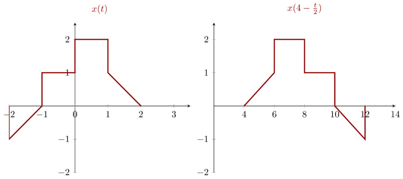
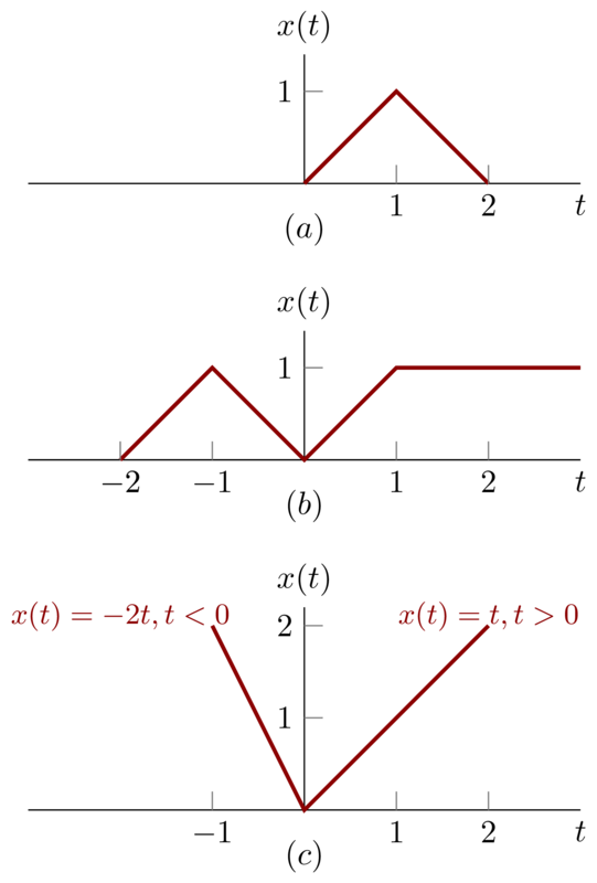
A continuout-time signal \(x(t)\) is shown below. Sketch and label carefully each of the following signals:
\begin{equation*}
\begin{array}{ll}
\mathbf{(a)}: x(t-1) & \mathbf{(b)}: x(2-t) \\
\mathbf{( c)}: x(2t + 1) & \mathbf{(d)}: x(4-\frac{t}{2}) \\
\mathbf{(e)}: [x(t) + x(-t)] u(t) & \mathbf{(f)}: x(t)\delta(t +\frac{3}{2}) - \delta(t-\frac{3}{2})
\end{array}
\end{equation*}
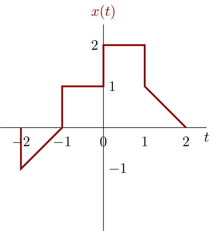
Before we figure all the sub-problem out. Let’s review how \(a\) and \(b\) affect \(x(at+b)\) . we know that:
- when \(|a| < 1\), \(x(t)\) will be linearly stretched;
- when \(|a|>1\), \(x(t)\) will be linearly compressed;
- when \(a < 0\), \(x(t)\) will be reversed;
- when \(b\neq 0\) , \(x(t)\) will be shifted in time.
- when \(a>0, b>0\), \(x(t)\) will be shifted left.
- when \(a>0,b<0\), \(x(t)\) will be shifted right.
- when \(a<0,b>0\), \(x(t)\) will be reversed first then shifted right.
- when \(a<0,b<0\), \(x(t)\) will be reversed first, then shifted left.
Problem 1.21a
Based on the conclusion given above, we know that \(x(t-1)\) can be obtained by right shifting \(x(t)\) with step \(1\). So the result can be visualized as follows.
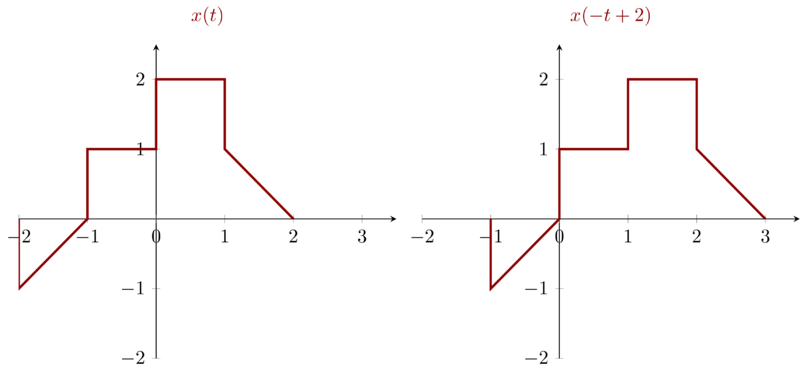
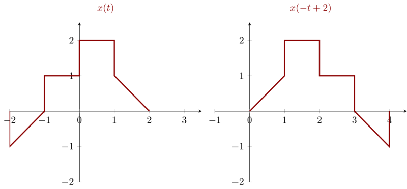
Problem 1.21b
For \(x(2-t)\), we re-write it as \(x(-(t-2))\) which can be obtained by first reversing \(x(t)\) then right shifting it with step \(2\). The result can be shown as follows
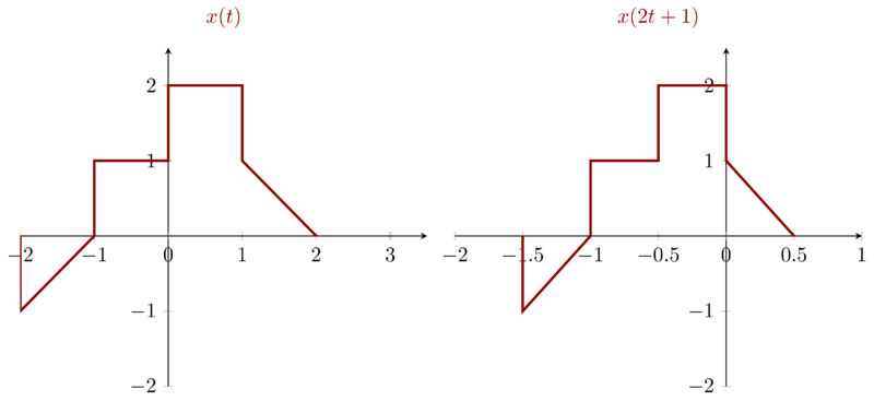
Problem 1.21c
\(x(2t + 1)\) can be re-written as \(x(2(t+\frac{1}{2}))\) which means that \(x(2t+1)\) can be obtained by first linearly compressing \(x(t)\) with factor 2 then left shifting compressed signal by \(\frac{1}{2}\).
Problem 1.21d
\(x(4-\frac{t}{2})\) can be re-written as \(x( -\frac{1}{2}( t - 8 ) )\) which means that \(x(4-\frac{t}{2})\) can be obtained by first linearly stretching \(x(t)\) by factor \(2\) then right shifting it with step \(8\).
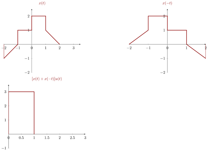
Problem 1.21e
At first glance, \(\big[x(t) + x(-t)\big] u(t) \) is \(0\) if \( t<0 \) .
If \( t > 0 \), we have to figure out \( x( -t ) \). After obtaining \( x(-t) \), we add the right part of \(x(t)\) and left part of \(x(-t)\) then we have \( [x(t) + x(-t)]u(t) \)
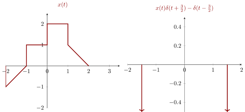
\(x(t)\delta(t +\frac{3}{2}) - \delta(t-\frac{3}{2})\) only have two points with non-negative values: \(t=\frac{3}{2}\) and \(t=-\frac{3}{2}\).
2 Problem 1.22
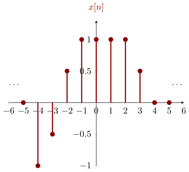
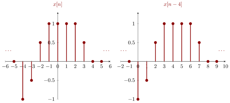
A discrete-time signal is shown in below figure. Sketch and label carefully each of the following signals:
\begin{equation*}
\begin{array}{ll}
\mathbf{(a)}: x[n-4] & \mathbf{(b)}: x[3-n] \\
\mathbf{( c)}: x[3n] & \mathbf{(d)}: x[3n + 1] \\
\mathbf{(e)}: x[n]u[3-n] & \mathbf{(f)}: x[n-2]\delta[n-2]\\
\mathbf{(g)}: \frac{1}{2}x[n] + \frac{1}{2}(-1)^{n}x[n] & \mathbf{(h)}: x[(n-1)^{2}]
\end{array}
\end{equation*}
Problem 1.22a
\(x[n-4]\) can be obtained by right shifting \(x[n]\) with step \(4\).
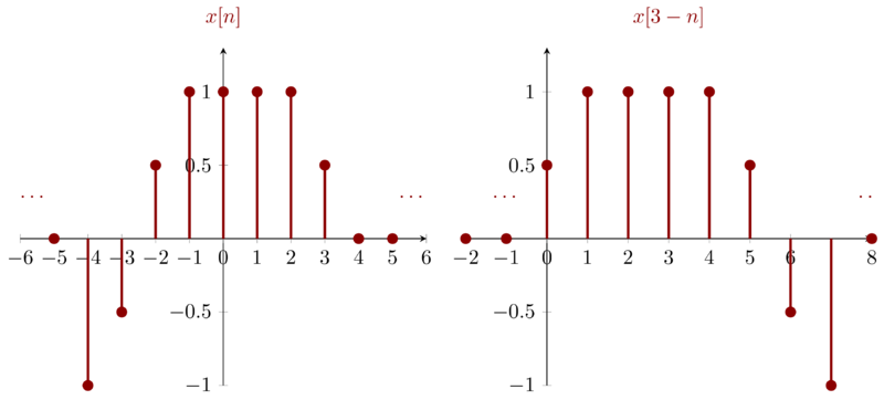
Problem 1.22b
\(x[3-n]\) can be obtained by reversing \(x[n]\) first then right shifting the reversed signal with step \(3\)
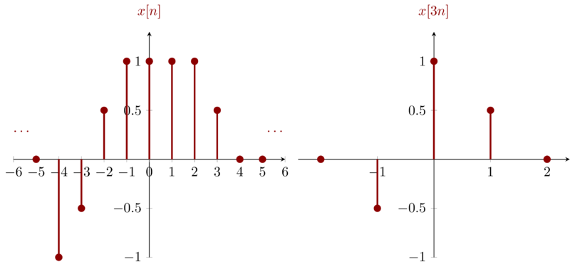
Problem 1.22c
\(x[3n]\) can be obtained by downsampling \(x[n]\) with a factor \(3\). Notice that downsampling discrete-time signal is different with compressing continuous-time signal because discrete-time signal only have integers as independent variables.
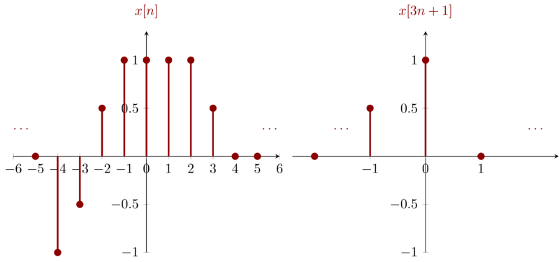
Problem 1.22d
\(x[3n+1]\) can be obtained by downsampling \(x[n]\) with a factor \(3\) and a delay \(1\).
Problem 1.22e
\(x[n]u[3-n]\) consists of two parts: \(x[n]\) and \(u[3-n]\). \(u[3-n]\), which can be obtained by reversing \(u[n]\) then right shifting \(3\) decides whether the result is zero or not.
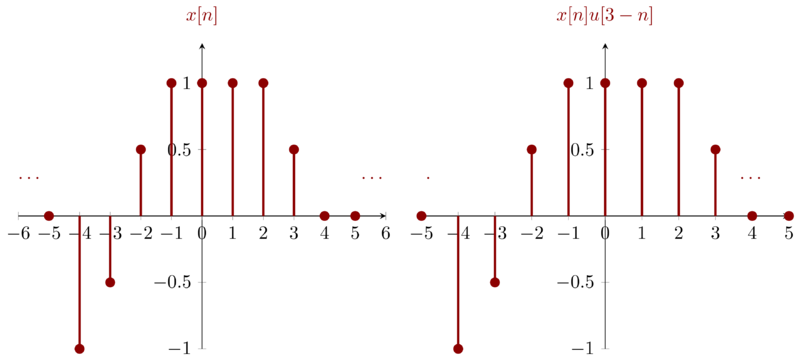
Notice that \(x[n]u[3-n]\) is the same as \(x[n]\) which is due to that \(u[3-n]\) is \(0\) if \(n>3\) and \(x[n]\) is also \(0\) if \(n>3\).
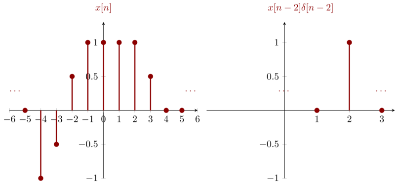
Problem 1.22f
\(x[n-2]\delta[n-2]\) can be obtained by sampling \(x[n]\) at \(n=2\).
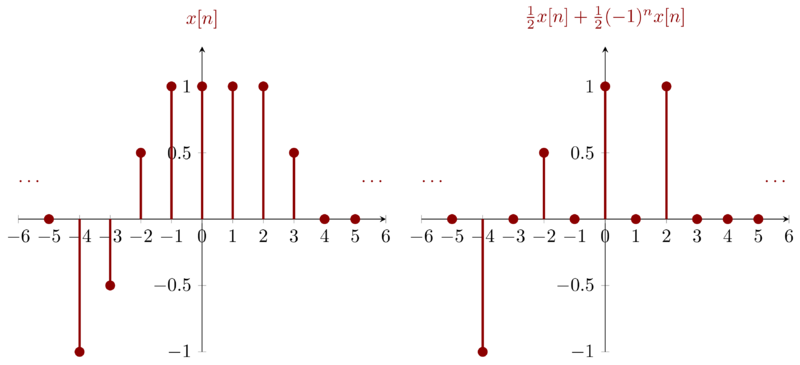
Problem 1.22g
\begin{equation*}
\frac{1}{2}x[n] + \frac{1}{2}(-1)^{n}x[n] =
\begin{cases}
0 & n \mathrm{\ is\ odd} \\
x[n] & n \mathrm{\ is\ even} \\
\end{cases}
\end{equation*}
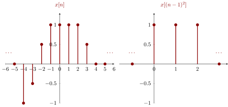
Problem 1.22h
\(x[(n-1)^{2}]\) can be obtained by sampling \(x[n]\) with sampling index \((n-1)^{2}\).
Let \(y[n] = x[(n-1)^{2}]\), we have
\begin{eqnarray*}
y[-1]&=&x[4] = 0 \\
y[0] &=&x[1] = 1 \\
y[1] &=&x[0] = 1 \\
y[2] &=&x[1] = 1 \\
y[3] &=&x[4] = 0
\end{eqnarray*}
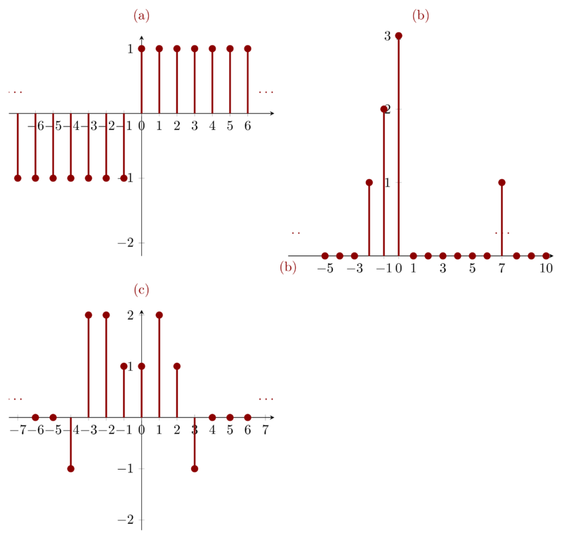
3 Problem 1.23
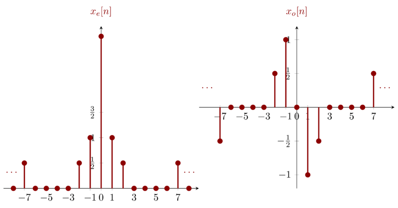
Determine and sketch the even and odd parts of the signals shown below. Label your sketches carefully
Before we figure them out, let’s review the definition of odd and even part of one signal.
Any signal can be seperated into two parts: the even part and the odd part.
\begin{eqnarray*}
x_{e}(t) = \mathrm{Even}\{x(t)\}&=& \frac{1}{2} [ x(t) + x(-t) ] \\
x_{o}(t) = \mathrm{Odd}\{x(t)\}&=& \frac{1}{2} [ x(t) - x(-t) ] \\
\end{eqnarray*}
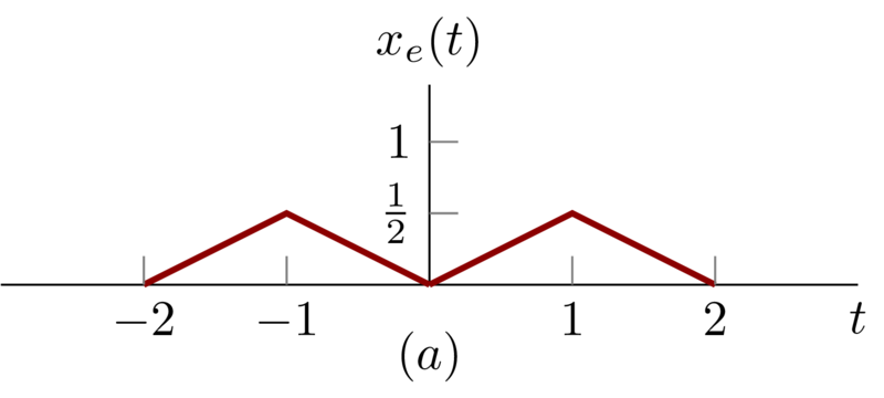
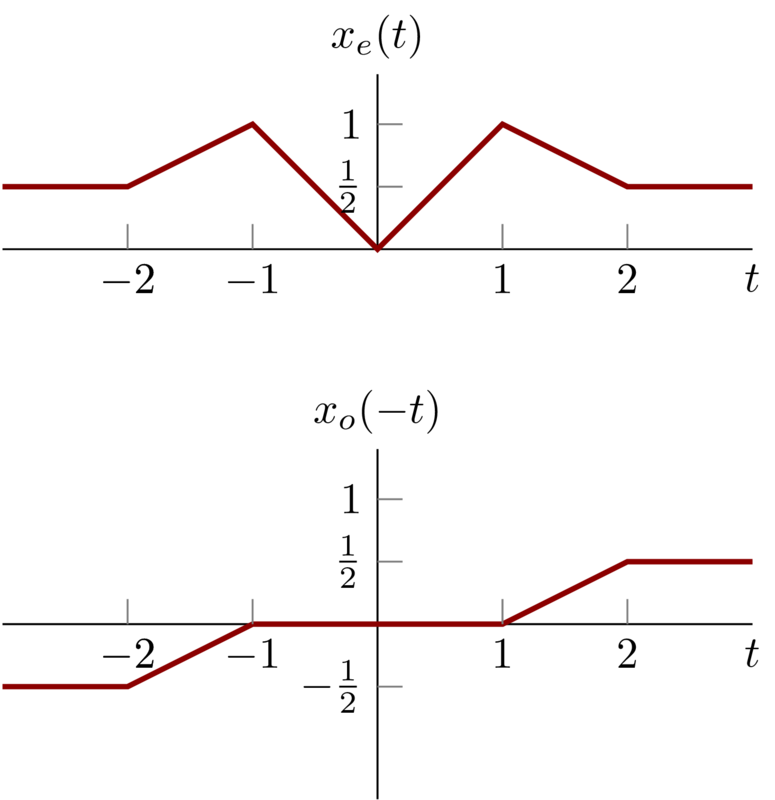
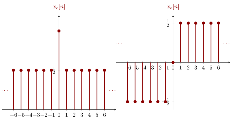
Problem 1.23a
If \(t\le 0\), we have \(x_{e}(t) = \frac{1}{2} x(-t) \) ;
if \(t > 0 \) , we have \(x_{e}(t) = \frac{1}{2} x(t) \); So, we illustrate \(x_{e}(t)\) as follows
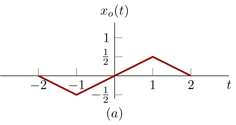
If \(t<0\), we have \(x_{o}(t) = - \frac{1}{2} x(-t) \) ;
if \(t > 0 \) , we have \(x_{o}(t) = \frac{1}{2} x(t) \); So, we illustrate \(x_{o}(t)\) as follows
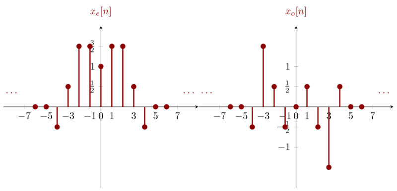
Problem 1.23b
To draw the \(x_{e}(t)\) , get \(\frac{1}{2} x(t)\) , \(\frac{1}{2}x(-t)\) and \(-\frac{1}{2}x(-t)\) first.
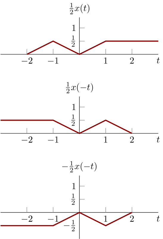
So we have \(x_{e}(t)\) and \(x_{o}(t)\) as below:
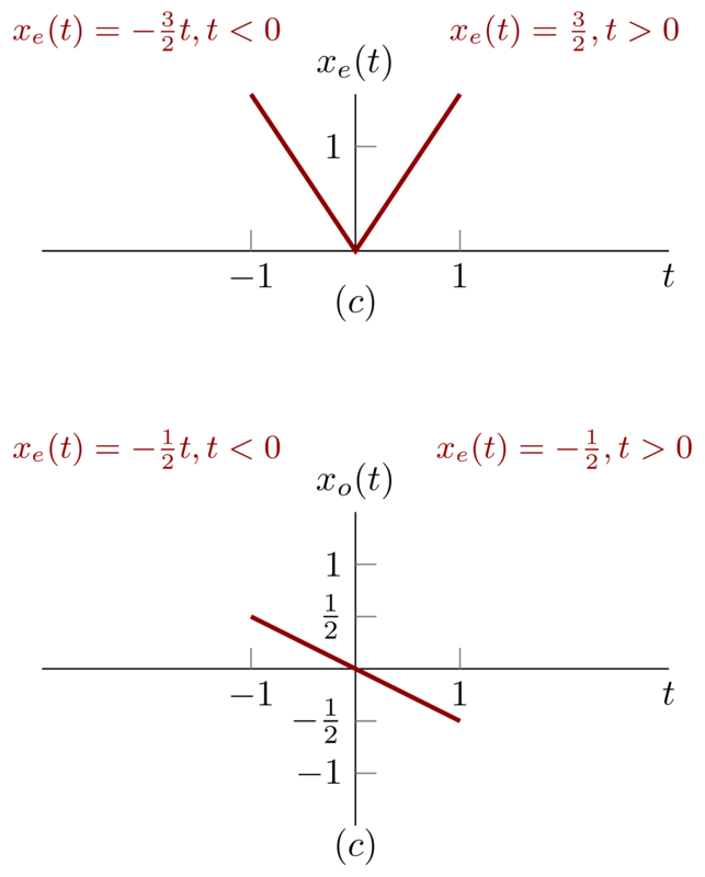
Problem 1.23c
I decide to figure this problem in a algebraic instead of geometrical way. because we have:
\begin{equation*}
x(t) =
\begin{cases}
-2t & t< 0\\
t & t > 0
\end{cases}
\end{equation*}
So
\begin{equation*}
x(-t) =
\begin{cases}
-t & t < 0 \\
2t & t> 0
\end{cases}
\end{equation*}
Then,
\begin{eqnarray*}
x_{e}(t)&=&
\begin{cases}
\frac{3}{2}t & t> 0\\
-\frac{3}{2}t & t < 0
\end{cases}
\\
x_{o}(t)&=&
\begin{cases}
-\frac{1}{2}t & t> 0\\
-\frac{1}{2}t & t< 0
\end{cases}
\end{eqnarray*}
Then we can draw them
4 Problem 1.24
Determine and sketch the even and odd parts of the signals depicted in the following figure. Label your sketches carefully
Based on the definition of even and odd parts of one signal and the analysis in Problem 1.23 , draw the result directly.
Problem 1-24a
Problem 1.24b
Problem 1-24c
5 Problem 1.25
Determine whether or not each of the following continuous-time signals is periodic. If the signal is periodic, determine its fundamental period.
\begin{eqnarray*}
\mathbf{(a)}: x(t) &=& 3\cos(4t + \frac{\pi}{3}) \\
\mathbf{(b)}: x(t) &=& e^{i( \pi t -1 )} \\
\mathbf{( c)}: x(t) &=& [\cos(2t - \frac{\pi}{3})]^{2} \\
\mathbf{(d)}: x(t) &=& \mathrm{Even}\{ \cos (4\pi t)u(t) \} \\
\mathbf{(e)}: x(t) &=& \mathrm{Even} \{\sin(4\pi t)u(t)\} \\
\mathbf{(f)}: x(t) &=& \sum_{n=-\infty}^{\infty} e^{-(2t -n)} u(2t-n)
\end{eqnarray*}
Problem 1.25a
The signal is periodic and the fundamental period \(T\) satisfies \(4T = 2\pi\) , so \(T = \frac{\pi}{2}\)
Problem 1.25b
The signal is periodic and the fundamental period \(T\) satisfies \(\pi T = 2\pi\), so \(T = 2\)
Problem 1.25c
To figure out whether or not the signal is periodic, we have to re-express the signal as:
\begin{eqnarray*}
\bigg[\cos(2t - \tfrac{\pi}{3})\bigg]^{2} &=& \bigg[ \frac{ e^{i(2t-\tfrac{\pi}{3}) } - e^{-i(2t - \tfrac{\pi}{3})} }{2} \bigg]^{2} \\
&=& \frac{1}{4} \bigg[ \frac{ e^{i2(2t-\tfrac{\pi}{3}) } + e^{-i2(2t - \tfrac{\pi}{3})} }{2} \bigg] \\
&=& \frac{1}{2} \big( 1 + \cos(4t - \tfrac{2\pi}{3}) \big)
\end{eqnarray*}
so the signal is periodic and the fundamental period \(T\) satisfies \(4T = 2\pi\) , so \(T = \frac{\pi}{2}\) .
Problem 1.25d
Because even part of \(\cos(4\pi t)u(t)\) is symmetrical about y-axis, the signal is periodic and the fundamental period \(T\) satisfies \(4\pi T = 2\pi \). So the fundamental period is \(T = \frac{1}{2}\)
Problem 1.25e
Because \(\sin(4\pi t)\) is an odd signal and \(\mathrm{Even} \{\sin(4\pi t)u(t)\}\) is symmetrical about y-axis. So the signal is not periodic.
Problem 1.25f
From the signal \(\mathbf{(f)}\) , we can see that there is no difference between whether \(n\) is \(n+1\) or \(n-1\) because \(n\) have value from \(-\infty\) to \(\infty\). So when we set \(n\) as \(n+1\), we have,
\begin{equation*} \sum_{n=-\infty}^{\infty} e^{-(2t -n-1)} u(2t-n-1) = \sum_{n=-\infty}^{\infty} e^{-(2t -n)} u(2t-n) \end{equation*}
Notice we can move the \(1\) in the left part of the above equation into \(t\) , so
\begin{equation*} \sum_{n=-\infty}^{\infty} e^{-(2( t -\tfrac{1}{2} ) -n)} u(2(t-\tfrac{1}{2})-n) = \sum_{n=-\infty}^{\infty} e^{-(2t -n)} u(2t-n) \end{equation*}
Because \(n\) must be integers, so \(1\) is the minimum value we can add to \(n\). Hence, the signal is periodic and its fundamental period is \(\frac{1}{2}\)
6 Problem 1.26
Determine whether or not each of the following discrete-time signals is periodic. If the signal is periodic, determine its fundamental period.
\begin{eqnarray*}
\mathbf{(a)}: x[n] &=& \sin (\frac{6\pi}{7}n +1) \\
\mathbf{(b)}: x[n] &=& \cos(\frac{n}{8} - \pi) \\
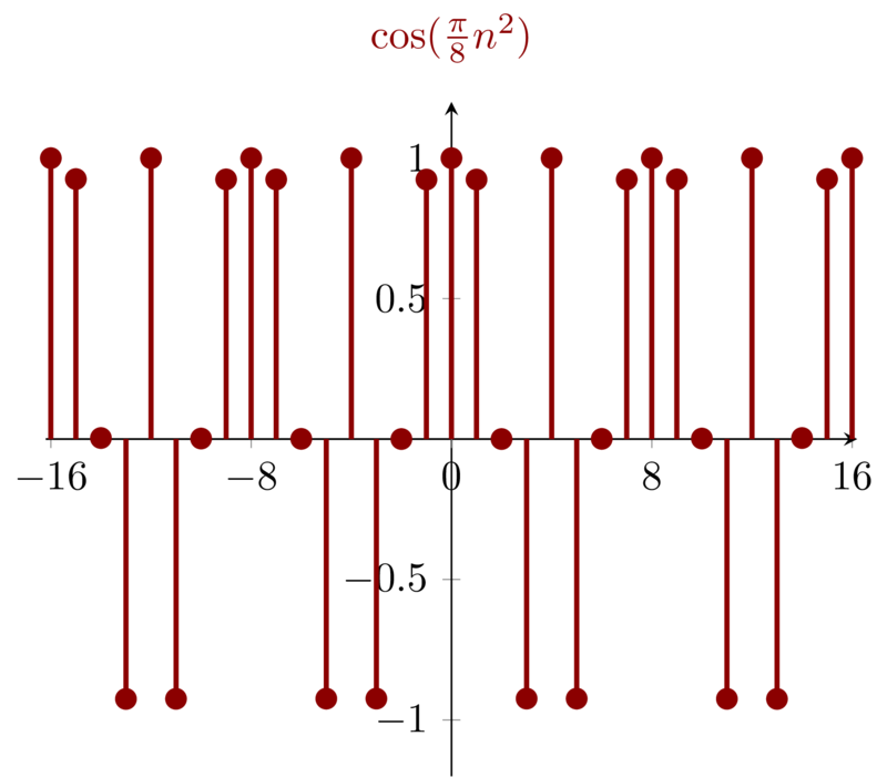
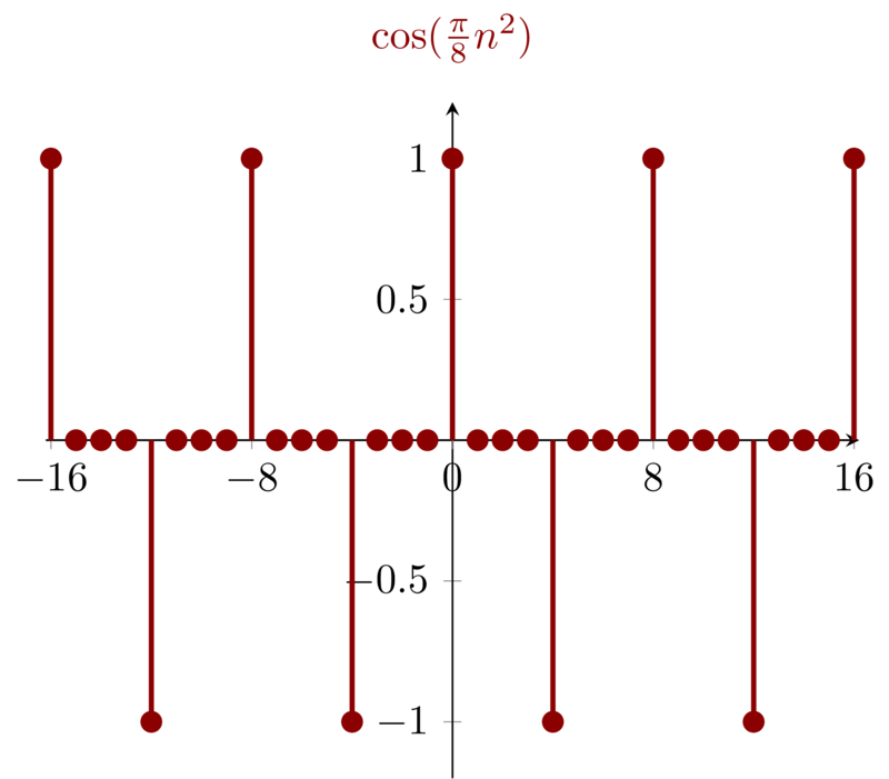
\mathbf{( c)}: x[n] &=& \cos(\frac{\pi}{8}n^{2}) \\
\mathbf{(d)}: x[n] &=& \cos(\frac{\pi}{2}n)\cos(\frac{\pi}{4}n) \\
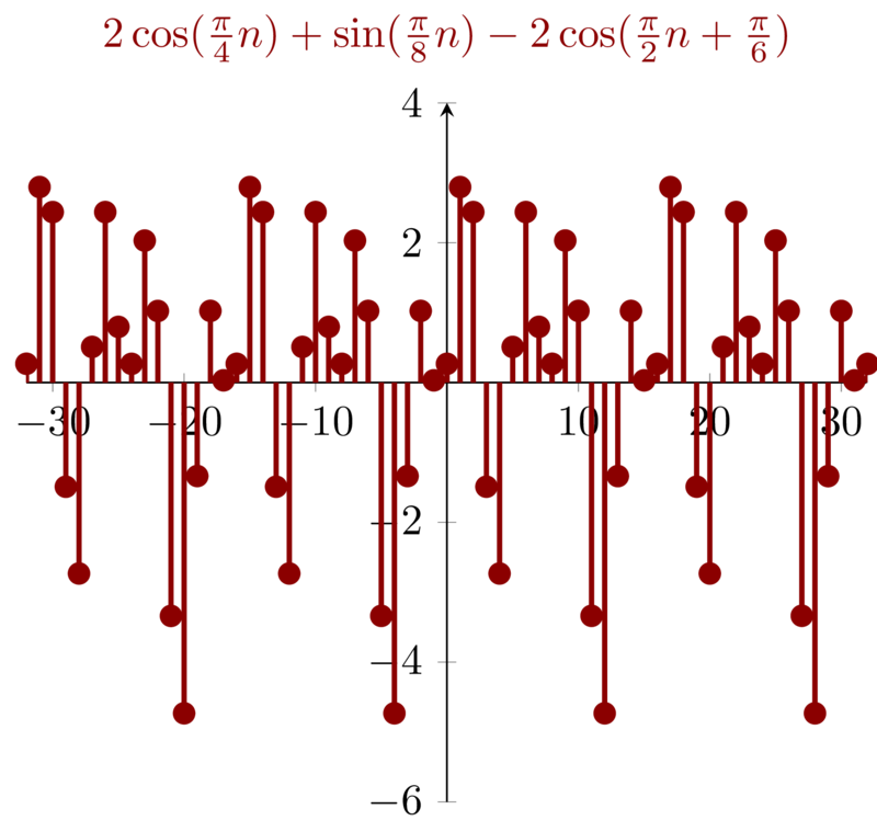
\mathbf{(e)}: x[n] &=& 2\cos(\frac{\pi}{4}n) + \sin(\frac{\pi}{8}n) - 2\cos(\frac{\pi}{2}n + \frac{\pi}{6})
\end{eqnarray*}
Suppose \(\mathbf{(a)}\) is periodic and the fundamental period is \(N\), so
\begin{equation*} \frac{6\pi}{7}N = m2\pi \end{equation*}
we have
\begin{equation*} N = m \frac{14}{3} \end{equation*}
Hence, signal \(\mathbf{(a)}\) is periodic and the fundamental period is \(14\) (when \(m=3\)).
Suppose signal \(\mathbf{(b)}\) is periodic and the fundamental period is \(N\), so
\begin{equation*} \frac{N}{8} = m2\pi \end{equation*}
we have,
\begin{equation*} N = 16m\pi \end{equation*}
So there is no interger \(m\) such that \(N\) is integer. So the signal is not periodic.
Suppose signal \(\mathbf{( c)}\) is periodic and the fundamental period is \(N\), we have
\begin{equation*} x[n+N] = \cos(\frac{\pi}{8} (n + N)^{2} ) = \cos(\frac{\pi}{8} ( n^{2} + 2nN + N^{2}) ) \end{equation*}
and \(x[n] = x[n+N]\), Then
\begin{equation*} \frac{\pi}{8}(2nN + N^{2}) = m2\pi \end{equation*}
which means that no matter what \(n\) is the equation must have interger \(m\) and \(N\). When \(N=8\) we have \(m\) as integer.
Both \(\cos(\frac{\pi}{2}n)\) and \(\cos(\frac{\pi}{4}n)\) are periodic with fundamental period \(4\) and \(8\) respectively. So the least common multiple of \(4,8\) will be the fundamental period of signal \(\mathbf{(d)}\). i.e. \(8\)
Problem 1.26e
Signal \(\mathbf{(e)}\) consists of three parts \( \cos(\frac{\pi}{4}n) \) , \(\sin(\frac{\pi}{8}n) \) and \(\cos(\frac{\pi}{2}n + \frac{\pi}{6})\) , with fundamental period \(8,16,4\) respectively. So the fundamental period is \(16\).
7 Problem 1.27
In this chapter, we introduced a number of general properities of systems. In particular, a system may or may not be
- Memoryless
- Time invariant
- Linear
- Causal
- Stable
Determine which of these properities hold and which do not hold for each of the following continuous-time systems. Justify your answers. In each example, \(y(t)\) denotes the system output and \(x(t)\) is the system input.
\begin{eqnarray*}
\mathbf{(a)} y(t)&=&x(t-1) + x(2-t) \\
\mathbf{(b)} y(t)&=&[\cos(3t)]x(t) \\
\mathbf{( c)} y(t)&=&\int_{-\infty}^{2t} x(\tau)\mathrm{d}\tau \\
\mathbf{(d)} y(t)&=&
\begin{cases}
0, & t < 0 \\
x(t) + x(t-2), & t\geq 0
\end{cases} \\
\mathbf{(e)} y(t) &=&
\begin{cases}
0, & x(t) < 0 \\
x(t) + x(t-2), & x(t)\geq 0
\end{cases} \\
\mathbf{( f )} y(t) &=& x(t/3) \\
\mathbf{(g)} y(t) &=& \frac{\mathrm{d}x(t)}{\mathrm{d}t}
\end{eqnarray*}
Memoryless : A system is memoryless if its output for each value of the independent variable at a give time is dependent on the input at only that same time.
Time invariant: A system is time invariant if the behavior and characteristics of the system are fixed over time. Time invariance can be justified very simply. A system is time invariant if a time shift in the input signal results in an identical time shift in the output signal.
Linear: A system is linear if it possesses the property of superposition: if an input consists of the weighted sum of several signals, then the output is the superposition.
Causality: A system is causal if the output at any time depends on values of the input at only the present and past time.
Stability: A system is stable if small inputs lead to response that do not diverge.
Problem 1.27a
- \(y(0)=x(-1) + x(2)\) , system \(\mathbf{(a)} \) has memory;
- If we delay the input by \(t_{0}\), then we have the output \(x(t -1-t_{0}) + x(2-t-t_{0})\); if we delay the output by \(t_{0}\), then we have the output \(y(t-t_{0}) = x(t-t_{0} -1) + x(2 - (t-t_{0}))\); system \(\mathbf{(a)}\) is time variant.
- System \(\mathbf{(a)}\) is not linear due to the counterexample \(x(t) = t^{2}\). If \( x(t) = t^{2} \), \(y(t) = t^{2} -6t + 5\) which is obviously not linear.
- Because \(y(0)=x(-1) + x(2)\), system \(\mathbf{(a)}\) is not causal.
- If \(|x(t)| < B\) , then \(|y(t)|< 2B \). System \(\mathbf{(a)}\) is stable.
Problem 1.27b
- The system is memoryless because the output only related with the current input.
- The system is time variant because the system has a time-varying gain with the input.
- The system is linear.
- The system is causal because the system is memoryless.
- The system is stable. If \(|x(t)| < B\), then \(|y(t)| < B\).
Problem 1.27c
- The system has memory because of the integration.
The system is time variant. Let \(x_{1}(t)\) be an arbitary signal, and \(y_{1}(t)\) the output. If we delay the input by \(t_{0}\) to get \(x_{2}(t) = x_{1}(t-t_{0})\), then the output should be:
\begin{eqnarray*} y_{2}(t)&=& \int_{-\infty}^{2t} x_{2}(\tau) \mathrm{d}\tau \\
&=& \int_{-\infty}^{2t} x_{1}(\tau - t_{0}) \mathrm{d}\tau \\
&=& \int_{-\infty}^{2t + t_{0}} x_{1}(\tau ) \mathrm{d}\tau \\
\end{eqnarray*}However, when we delay the \(y_{1}(t)\) by \(t_{0}\), we get
\begin{eqnarray*} y_{1}(t - t_{0})&=& \int_{-\infty}^{2(t-t_{0})} x_{1}(\tau ) \mathrm{d}\tau \\
&\neq& y_{2}(t) \end{eqnarray*}The system is linear because of integration.
The system is not causal because \(y(t)\) is related with \(x(2t)\).
The system is not stable because of the existence of \(-\infty\).
Problem 1.27d
- The system has memory. because \(y(4) = x(4) + x(2)\)
- The system is time variant. because when \(t<0\) the output is \(0\). If we shift the time to make \(t\geq 0\), then the output \(y(t)\) is \(x(t) + x(t-2)\) which is possible not \(0\). i.e. a time shift in the input signal does not result in an identical time shift in the output signal.
- The system is linear.
- The system is causal because the current output only related with current or past input.
- The system is stable.
Problem 1.27e
- The system has memory.
- The system is time invariant. because a time shift in the input signal will definitely result an identical shift in the output. Notice carefully that the system is defined only relating with \(x(t)\) instead of \(t\) as in system \(\mathbf{(d)}\).
- The system is linear.
- The system is causal because the output only relate with the current and the past input.
- The system is stable.
Problem 1.27f
- The system has memory.
- The system is time variant.
- The system is linear.
- The system is not causal, because \(y(-1) = x(-\frac{1}{3})\).
- The system is stable.
Now, I justify the properity of time variant of system \(\mathbf{(f)}\). Let arbitary input \(x_{1}(t)\) and the output \(y_{1}(t) = x_{1}(\tfrac{t}{3})\). Let \(x_{2}(t) = x_{1}(t - t_{0})\), then \(y_{2}(t) = x_{2}(\tfrac{t}{3}) = x_{1}( \frac{t}{3} - t_{0} )\) which is not equal with \(y_{1}(t-t_{0}) = x(\frac{t-t_{0}}{3})\) .
Problem 1.27g
- The system has memory by definition of diffenence.
- The system is time invariant.
- The system is linear
- The system is causal.
- The system is not stable. For some signal \(x(t)\) with certain \(t\) the signal is not differentiable.
8 Problem 1.28
Determine which of the properties listed in Problem 1.27 hold and which do not hold for each of the following discrete-time systems. Justify your answers. In each example, \(y[n]\) denotes the system output and \(x[n]\) is the system input.
\begin{eqnarray*}
\mathbf{(a)} y[n]&=& x[-n] \\
\mathbf{(b)} y[n]&=& x[n-2] -2x[n-8] \\
\mathbf{( c)} y[n]&=& nx[n] \\
\mathbf{(d)} y[n]&=& \mathrm{Even} \{ x[n-1] \} \\
\mathbf{(e)} y[n]&=&
\begin{cases}
x[n], & n\geq 1\\
0, & n=0 \\
x[n+1], & n\leq -1
\end{cases} \\
\mathbf{(f)} y[n] &=&
\begin{cases}
x[n], & n\geq 1\\
0, & n=0 \\
x[n], & n\leq -1
\end{cases} \\
\mathbf{(g)} y[n] &=& x[4n+1]
\end{eqnarray*}
Memoryless : A system is memoryless if its output for each value of the independent variable at a give time is dependent on the input at only that same time.
Time invariant: A system is time invariant if the behavior and characteristics of the system are fixed over time. Time invariance can be justified very simply. A system is time invariant if a time shift in the input signal results in an identical time shift in the output signal.
Linear: A system is linear if it possesses the property of superposition: if an input consists of the weighted sum of several signals, then the output is the superposition.
Causality: A system is causal if the output at any time depends on values of the input at only the present and past time.
Stability: A system is stable if small inputs lead to response that do not diverge.
Problem 1.28a
- The system has memory.
- The system time variant.
- The system is linear.
- The system is not causal because \(y[-2]=x[2]\)
- The system is stable.
Now, Let me justify the property of time variant. Let \(x_{1}[n]\) be an arbitary singal and hence the output \(y_{1}[n] = x_{1}[-n]\). Let \(x_{2}[n] = x_{1}[n-n_{0}]\) and hence \(y_{2}[n] = x_{2}[-n] = x_{1}[-n-n_{0}]\) which is not equal with \(y_{1}[n-n_{0}] = x_{1}[-(n-n_{0})]\). Hence, the time shift in the input signal does not result in the same time shift in the output signal.
The process of justifing can be visualized as below:
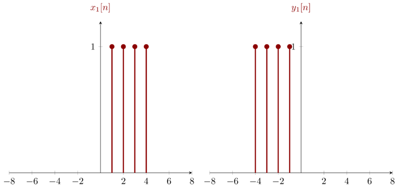
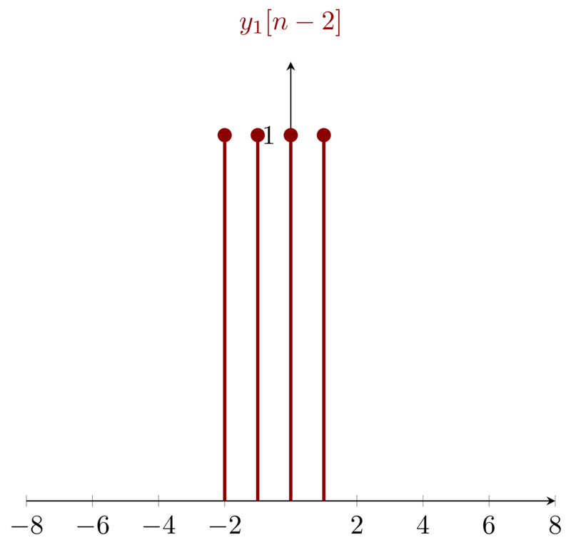
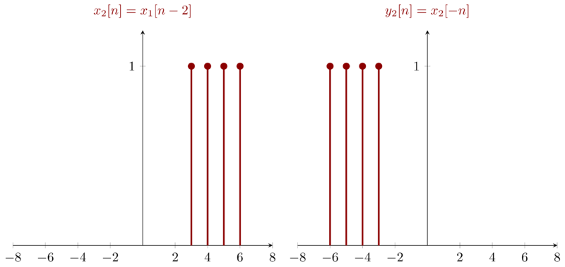
As we can see \(y_{2}[n]\neq y_{1}[n-2]\) i.e. the time shift ( here \(2\)) in input signal does not result in the identical time shift in the result.
Problem 1.28b
- The system has memory.
- The system is time invariant.
- The system is linear.
- The system is causal.
- The system is stable.
Problem 1.28c
- The system is memoryless.
- The system is time variant.
- The system is linear.
- The system is causal.
- The system is not stable.
Problem 1.28d
- The system has memory.
- The system is time variant.
- The system is linear.
- The system is not causal.
- The system is stable.
Problem 1.28e
- The system has memory.
- The system is time variant
- The system is linear.
- The system is not causal.
- The system is stable.
Problem 1.28f
- The system has no memory.
- The system is time variant.
- The system is linear.
- The system is causal.
- The system is stable.
Problem 1.28g
- The system has memory.
- The system is time variant.
- The system is linear.
- The system is not causal.
- The system is stable.
9 Problem 1.29
- Show that the discrete-time system whose input \(x[n]\) and output \(y[n]\) are related by \(y[n] = \mathrm{Re} \{x[n]\} \) is additive. Does this system remain additive if its input-output relationship is changed to \(y[n] = \mathrm{Re} \{ e^{i\pi n/4}x[n] \} \)? (Do not assume that \(x[n]\) is real in this problem.)
In the text, we discussed the fact that the property of linearity for a system is equivalent to the system possessing both the additive property and homogeneity property. Determine whether each of the systems defined below is additive and/or homogeneous. Justify your answers by providing a proof for each property if it holds or a counterexample if it does not.
\begin{eqnarray*} \mathrm{(i)}: y(t) &=&\frac{1}{x(t)} \big[ \frac{dx(t)}{dt} \big]^{2} \\
\mathrm{(ii)}: y[n] &=& \begin{cases} \frac{x[n]x[n-2]}{x[n-1]}, & x[n-1] \neq 0 \\
0, & x[n-1] = 0 \end{cases} \end{eqnarray*}
Problem 1.29a
Let \(x[n] = x_{r}[n] + i x_{i}[n]\) where \(x_{r}[n]\) and \(x_{i}[n]\) stand for the real part and imagary part of \(x[n]\) respectively. Let \(x_{1}[n] = x_{1r}[n] + ix_{1i}[n]\) and \(x_{2}[n] = x_{2r}[n] + i x_{2i}[n]\), so \(y_{1}[n] = \mathrm{Re} \{x_{1}[n]\} = x_{1r}[n]\) and \(y_{2}[n] = \mathrm{Re}\{x_{2}[n]\} =x_{1r}[n] \). Let \(x_{3}[n] = x_{1}[n] + x_{2}[n] = ( x_{1r}[n] + x_{2r}[n]) + i( x_{1i}[n] + x_{2i}[n] )\). Then we have \(y_{3}[n] = x_{1r}[n] + x_{2r}[n] = y_{1}[n] + y_{2}[n]\). So the the relationship \(y[n] = \mathrm{Re}\{ x[n]\}\) between \(x[n]\) and \(y[n]\) is additive.
Next Let’s check whether or not the additive property of \(y[n] =\mathrm{Re} \{ e^{i\pi n/4}x[n] \} \) holds. First Let \(x[n] = x_{r}[n] + ix_{i}[n]\) like before. Then,
\begin{eqnarray*}
y[n]&=& \mathrm{Re} \{ e^{i\pi n/4}x[n] \} \\
&=& \mathrm{Re} \{ (\cos(\tfrac{\pi n}{4} ) + i\sin(\tfrac{\pi n}{4})) ( x_{r}[n] + ix_{i}[n] ) \} \\
&=& \cos(\tfrac{\pi n}{4})x_{r}[n] -\sin( \tfrac{\pi n}{4} )x_{i}[n]
\end{eqnarray*}
The additive property holds in a straightforward way.
Problem 1.29b(i)
First let’s check whether the additive property holds or not. Suppose
\begin{eqnarray*}
y_{1}(t)&=& \frac{1}{x_{1}(t)} \big[ \frac{dx_{1}(t)}{dt} \big]^{2} \\
y_{2}(t)&=& \frac{1}{x_{2}(t)} \big[ \frac{dx_{2}(t)}{dt} \big]^{2} \\
\end{eqnarray*}
and \(x_{3}(t) = x_{1}(t) + x_{2}(t)\), then,
\begin{eqnarray*}
y_{3}(t)&=& \frac{1}{x_{3}(t)} \big[ \frac{dx_{3}(t)}{dt} \big]^{2} \\
&=& \frac{1}{x_1(t) + x_2(t)} \big[ \frac{d( x_1(t) + x_2(t) )}{dt} \big]^{2} \\
&\neq& y_{1}(t) + y_{2}(t)
\end{eqnarray*}
So the additive property does not holds.
Second, let’s check the property of homogeneity. Suppose \(x_{4}(t) = ax_{1}(t)\), then
\begin{eqnarray*}
y_{4}(t)&=& \frac{1}{x_{4}(t)} \big[ \frac{dx_{4}(t)}{dt} \big]^{2} \\
&=& \frac{1}{ax_{1}(t)} \big[ \frac{dax_{1}(t)}{dt} \big]^{2} \\
&=& a\frac{1}{x_{1}(t)} \big[ \frac{dx_{1}(t)}{dt} \big]^{2} \\
&=& ay_{1}(t)
\end{eqnarray*}
So the homogeneity property holds.
Problem 1.29b(ii)
Let
\begin{eqnarray*}
y_{1}[n] &=&
\begin{cases}
\frac{x_{1}[n]x_{1}[n-2]}{x_{1}[n-1]}, & x_{1}[n-1] \neq 0 \\
0, & x_{1}[n-1] = 0
\end{cases} \\
y_{2}[n] &=&
\begin{cases}
\frac{x_{2}[n]x_{2}[n-2]}{x_{2}[n-1]}, & x_{2}[n-1] \neq 0 \\
0, & x_{2}[n-1] = 0
\end{cases}
\end{eqnarray*}
and let \(x_{3}[n] = x_{1}[n] + x_{2}[n]\), we have
\begin{eqnarray*}
y_{3}[n] &=&
\begin{cases}
\frac{x_{3}[n]x_{3}[n-2]}{x_{3}[n-1]}, & x_{3}[n-1] \neq 0 \\
0, & x_{3}[n-1] = 0
\end{cases} \\
&=&
\begin{cases}
\frac{(x_1[n]+x_2[n]) ( x_{1}[n-2] + x_{2}[n-2] )}{x_{1}[n-1] + x_{2}[n-1]}, & x_{1}[n-1] + x_{2}[n-1]\neq 0 \\
0, & x_{1}[n-1] + x_{2}[n-1]= 0
\end{cases}
\end{eqnarray*}
We cannot reach the conclusion that \(y_{3}[n]= y_{1}[n] + y_{2}[n]\). So the additive property does not hold.
Second Let’s check whether the homogeneity property holds. Let \(x_{4}[n] = ax_{1}[n]\) , It’s easy to check the system is homogeneous. i.e. \(y_{4}[n] = ay_{1}[n]\)
10 Problem 1.30
Determine if each of the following systems is invertible. If it is, construct the inverse system. If it is not, find two input signals to the system that have the same output.
\begin{eqnarray*}
\mathbf{(a)} y(t)&=&x(t-4) \\
\mathbf{(b)} y(t)&=&\cos[x(t)] \\
\mathbf{( c)} y(t)&=&nx[n] \\
\mathbf{(d)} y(t)&=&\int_{-\infty}^{t} x(\tau)d\tau \\
\mathbf{(e)} y[n]&=&
\begin{cases}
x[n-1], & n\geq 1 \\
0, & n=0 \\
x[n], & n\leq -1
\end{cases} \\
\mathbf{(f)} y[n]&=& x[n]x[n-1] \\
\mathbf{(g)} y[n]&=& x[1-n] \\
\mathbf{(h)} y(t)&=& \int_{-\infty}^{t} e^{-(t-\tau)}x(\tau)d\tau \\
\mathbf{(i)} y[n] &=& \sum_{k=-\infty}^{n}(\tfrac{1}{2})^{n-k}x[k] \\
\mathbf{(j)} y(t) &=& \frac{dx(t)}{dt} \\
\mathbf{(k)} y[n] &=&
\begin{cases}
x[n+1] ,& n\geq 0 \\
x[n], & n\leq -1
\end{cases}\\
\mathbf{(l)} y(t) &=& x(2t) \\
\mathbf{(m)} y[n] &=& x[2n] \\
\mathbf{(n)} y[n] &=&
\begin{cases}
x[n/2], & n\ \mathrm{even} \\
0, & n\ \mathrm{odd}
\end{cases}
\end{eqnarray*}
A system is invertible if distinct inputs lead to distinct outputs. There exists an inverse system for an invertible system so that when cascaded with the original system, the output will be equal to the input to the original system.
Problem 1.30a
For system \(\mathbf{(a)}\), the output is the input delayed by \(4\), so the inverse system should be a system that advance the input by \(4\), i.e.
\begin{equation*} y(t) = x(t+4) \end{equation*}
Problem 1.30b
For system \(\mathbf{(b)}\), \(\cos(t)\) is and periodic signal with fundamental period \(2\pi\) which means that different inputs will lead to one same output. So the system may not be invertible.
Problem 1.30c
\(\delta[n]\) and \(2\delta[n]\) lead to the same result. So the system is not invertible.
The integration is invertible and the inverse system is
\begin{equation*} y(t) = \frac{dx(t)}{dt} \end{equation*}
Notice that the difference is not invertible like system \(\mathbf{(j)}\), because \(\frac{d(x(t) + t_{0})}{dt}\) will lead to the same result no matter what value \(t_{0}\) will be.
Like system \(\mathbf{(a)}\), this discrete-time system is invertible and the inverse system is
\begin{equation*}
y[n]=
\begin{cases}
x[n+1], & n\geq 1 \\
0, & n=0 \\
x[n], & n\leq -1
\end{cases} \\
\end{equation*}
Problem 1.30f
This system is not invertible. Let \(x[n] = \delta[n]\) and \(x[n] = \delta[n-1]\), we have the same output.
Problem 1.30g
\(y[n]\) is obtained by first flipping \(x[n]\) the right shifting the flipped signal by one. So we have the inverted system as \(y[n] = x[-n+1]\)
Problem 1.30h
The system is invertible and the inverse system is \(y(t)= x(t) + \frac{dx(t)}{dt}\)
Problem 1.30i
The system is invertible. First let’s re-express the original system as:
\begin{eqnarray*}
y[n] &=& \sum_{k=-\infty}^{n}(\tfrac{1}{2})^{n-k}x[k] \\
&=& \sum_{k=-\infty}^{n-1} ( \frac{1}{2} )^{n-k} x[k] + x[n]
\end{eqnarray*}
Then, we have \(x[n] = y[n] - \frac{1}{2}\sum_{k=-\infty}^{n-1} ( \frac{1}{2} )^{n-1-k} x[k] = y[n] - \frac{1}{2} y[n-1] \) So the inverse system is \( y[n]= x[n] - \frac{1}{2} x[n-1] \) So the inverse system is \( y[n]= x[n] - \frac{1}{2} x[n-1] \).
Problem 1.30j
The system is not invertible because \(x(t)\) and \(x(t) + x_{0}\) will result the same \(y(t)\). \(x_{0}\) is a constant.
Problem 1.30k
The system is not invertible. \(\delta[n]\) and \(2\delta[n]\) will result in same result.
Problem 1.30l
The system is invertible and the inverse system is \( y(t) = x(\frac{1}{2}t)\).
Problem 2.30m
The system is not invertible. Notice this system is different with system \(\mathbf{(l)}\) which is continuous-time system. \(x[2n]\) is a downsampling of \(x[n]\). So there are tons of signals as \(x[n]\) which can be downsampling to get \(x[2n]\).
Problem 2.30n
The system is invertible and the system is \(y[n] = x[2n]\)
11 Problem 1.31
In this problem, we illustrate one of the most important consequences of the properties of linearity and time invariance. Specifically, once we know the response of a linear system or a linear time-invariant (LTI) system to a single input or the response to several inputs, we can directly compute the response to many other input signals. Much of the remainder of this book deals with a thorough exploitation of this fact in order to develop results and techniques for analyzing and synthesizing LTI systems.
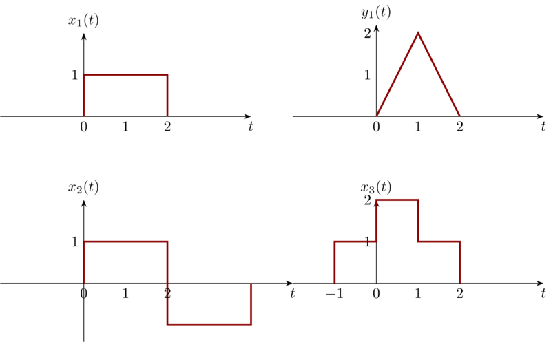
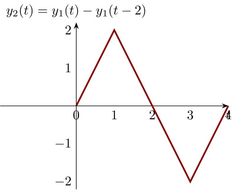
- Consider an LTI system whose response to the signal \(x_{1}(t)\) in the following figure is the signal \(y_{1}(t)\). Determine and sketch carefully the response of the system to the input \(x_{2}(t)\) .
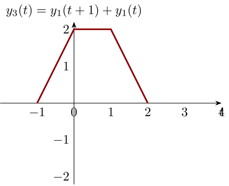
- Determine and sketch the response of the system considered in part (a) to the input \(x_{3}(t)\).
Problem 1.31a
Notice that \(x_{2}(t) = x_{1}(t) - x_{1}(t-2)\). Based on the properties of LTI system , we have \(y_{2}(t) = y_{1}(t) - y_{1}(t-2)\).
Notice that \(x_{3}(t) = x_{1}(t+1) + x_{1}(t)\). So the output \(y_{3}(t) =y_{1}(t+1) + y_{1}(t)\).
12 Reference
Bibliography
[oppenheim_signals_1997] Oppenheim, Signals and Systems, Prentice Hall (1997). ↩
MSC
Make STEAM Clear
I post articles and make videos about STEAM and try to explain the concepts in a more approachable and beautiful way.