Signals and Systems Chapter 1 Problems Part 3 (1.32-1.47)

- 1 Problem 1.32
- 2 Problem 1.33
- 3 Problem 1.34
- 4 Problem 1.35
- 5 Problem 1.36
- 6 Problem 1.37
- 7 Problem 1.38
- 8 Problem 1.39
- 9 Problem 1.40
- 10 Problem 1.41
- 11 Problem 1.42
- 12 Problem 1.43
- 13 Problem 1.44
- 14 Problem 1.45
- 15 Problem 1.46
- 16 Problem 1.47
1 Problem 1.32
Let \(x(t)\) be a continuous-time signal, and let
\begin{equation*} y_{1}(t) = x(2t) \ \mathrm{and} \ y_{2}(t) = x(t/2) \end{equation*}
The signal \(y_{1}(t)\) represents a speeded up version of \(x(t)\) in the sense that the duration of the signal is cut in half. Similarly, \(y_{2}(t)\) represents a slowed down version of \(x(t)\) in the sense that the duration of the signal is doubled. Consider the following statements:
- If \(x(t)\) is periodic, then \(y_{1}(t)\) is periodic.
- If \(y_{1}(t)\) is periodic, then \(x(t)\) is periodic.
- If \(x(t)\) is periodic, then \(y_{2}(t)\) is periodic.
- If \(y_{2}(t)\) is periodic, then \(x(t)\) is periodic.
For each of these statements, determine whether it is true, and if so, determine the relationship between the fundamental periods of the two signals considered in the statement. If the statement is not true, produce a counterexample to it.
Let \(T\) be the fundamental period of \(x(t)\), then we have \(x(t+T) = x(t)\). So \( y_{1}(t) = x(2t) = x(2t + T) = x(2(t+ \frac{T}{2} ))= y_{1}(t+\frac{T}{2})\), \(y_{1}(t)\) is periodic and the fundamental period is \( \frac{T}{2} \) which is consistent with our commonsense that \(y_{1}(t)\) is an speeded up version of \(x(t)\).
Problem 1.32b
Let \(T\) be the fundamental period of \(y_{1}(t)\), then based on the analysis of Problem 1.32a , we have \(x(t)\) is a slowed down version of \(y_{1}(t)\), hense \(x(t)\) is periodic and has fundamental period \(2T\).
Let \(T\) be the fundamental period of \(x(t)\), then we have \(x(t+T) = x(t)\). So \( y_{2}(t) = x(\tfrac{t}{2}) = x(\tfrac{t}{2} + T) = x(\frac{t+ 2T}{2})= y_{2}(t+2T)\), \(y_{2}(t)\) is periodic and the fundamental period is \(2T \) which is consistent with our commonsense that \(y_{2}(t)\) is an slowed down version of \(x(t)\).
Problem 1.32d
Let \(T\) be the fundamental period of \(y_{2}(t)\), then based on the analysis of Problem 1.32c , we have \(x(t)\) is a speeded up version of \(y_{2}(t)\), hense \(x(t)\) is periodic and has fundamental period \(\frac{T}{2}\).
2 Problem 1.33
Let \(x[n]\) be a discrete-time signal, and let
\begin{equation*}
y_{1}[n] = x[2n] \ \mathrm{and}\ y_{2}[n] =
\begin{cases}
x[n/2], & n\ \mathrm{even} \\
0, & n\ \mathrm{odd}
\end{cases}
\end{equation*}
The signals \(y_{1}[n]\) and \(y_{2}[n]\) respectively represent in some sense the speeded up and slowed down versions of \(x[n]\). However, it should be noted that the discrete-time notions of speeded up and slowed down have subtle differences with respect to their continuous-time counterparts. Consider the following statements:
- If \(x[n]\) is periodic, then \(y_{1}[n]\) is periodic.
- If \(y_{1}[n]\) is periodic, then \(x[n]\) is periodic.
- If \(x[n]\) is periodic, then \(y_{2}[n]\) is periodic.
- If \(y_{2}[n]\) is periodic, then \(x[n]\) is periodic.
Problem 1.33a
Let \(N\) be the fundamental period of \(x[n]\), then \(x[n+N] = x[n]\), and \(y_{1}[n] = x[2n] = x[2n+N] = y_{1}[n+ \frac{N}{2}]\). If \(N\) is even, then \(y_{1}[n]\) has fundamental period \(\frac{N}{2}\). It is a little tricky that when \(N\) is odd \(\frac{N}{2}\) has no meaning. If \(N\) is odd, we have to express \(y_{1}[n] = x[2n] = x[2n+2N] = y_{1}[n+ N]\) hence \(y_{1}[n]\) has fundamental period \(N\) if \(N\) is odd.
Problem 1.33b
We can see \(y_{1}[n]\) is not only a speeded up version but also a down sampling version of \(x[n]\). we cannot determine whether or not \(y_{1}[n]\) is periodic based on that \(x[n]\) is periodic. We can only tell that the even indexed value of \(x[n]\) is period. we know nothing about the odd indexed value of \(x[n]\). An example is given below:
The given \(x[n]\) is periodic at \(2n\) but is random at \(2n+1\).
\(y_{2}[n]\) can treated as interpolation of \(x[n]\) with zero. So \(y_{2}[n]\) is periodic with fundamental period \(2N\) where \(N\) is fundamental period of \(x[n]\).
Problem 1.33d
Based on analysis of Problem 1.33c , \(y_{2}[n]\) has fundamental period \(2N\) where \(N\) is the fundamental period of \(x[n]\).
Based on the fact that only integer is valid for the independent variable of discrete-time signal, \(y_{2}[n]\) contains all the value of \(x[n]\) at the even index whereas at the odd index \(y_{2}[n]= 0\).
3 Problem 1.34
In this problem, we explore several of the properties of even and odd signals.
Show that if \(x[n]\) is an odd signal, then
\begin{equation*} \sum_{n=-\infty}^{+\infty} x[n] =0 \end{equation*}
Show that if \(x_{1}[n]\) is an odd signal and \(x_{2}[n]\) is an even signal, then \(x_{1}[n]x_{2}[n]\) is an odd signal.
Let \(x[n]\) be an arbitrary signal with even and odd parts denoted by
\begin{equation*} x_{e}[n] = \mathrm{Even}\{ x[n] \} \end{equation*}
and
\begin{equation*} x_{o}[n] = \mathrm{Odd} \{ x[n] \} \end{equation*}
Show that
\begin{equation*} \sum_{n=-\infty}^{+\infty} x^{2}[n] = \sum_{n=-\infty}^{+\infty} x_{e}^{2}[n] + \sum_{n=-\infty}^{+\infty} x_{o}^{2}[n] \end{equation*}
Although parts 1-3 have been stated in terms of discrete-time signals, the analogous properties are also valid in continuous time. To demonstrate this, show that
\begin{equation*} \int_{-\infty}^{+\infty}x^{2}(t)dt = \int_{-\infty}^{+\infty} x_{e}^{2}(t)dt + \int_{-\infty}^{+\infty} x_{o}^{2}(t)dt \end{equation*}
where \(x_{e}(t)\) and \(x_{o}(t)\) are, respectively, the even and odd parts of \(x(t)\).
Problem 1.34a
If \(x[n]\) is an odd signal, then we have \(x[n] = -x[-n]\) and \(x[0]=0 \), so
\begin{eqnarray*}
\sum_{n=-\infty}^{+\infty} x[n] &=& \sum_{n=0}^{+\infty} x[n] + \sum_{-\infty}^{0} x[n] \\
&=& \sum_{n=0}^{\infty} \big( x[n] + x[-n] \big) \\
&=& 0
\end{eqnarray*}
Problem 1.34b
Because \(x_{1}[n]\) is an odd signal, \(x_{1}[n] = -x_{1}[-n]\). Because \(x_{2}[n]\) is an even signal, \(x_{2}[n] = x_{2}[-n]\). we have
\begin{equation*}
x_{1}[n]x_{2}[n] = -x_{1}[-n]x_{2}[-n] \\
\end{equation*}
i.e. \(x_{1}[n]x_{2}[n]\) is an odd signal.
Problem 1.34c
\begin{eqnarray*}
x_{e}[n] &=& \frac{x[n] + x[-n]}{2} \\
x_{o}[n] &=& \frac{x[n] - x[-n]}{2}
\end{eqnarray*}
Then we have
\begin{eqnarray*}
\sum_{n=-\infty}^{+\infty} x_{e}^{2}[n] &=& \sum_{n=-\infty}^{+\infty} \bigg( \frac{ x[n] + x[-n] }{2} \bigg)^{4} \\
&=& \sum_{n=-\infty}^{+\infty} \bigg( \frac{ x^{2}[n] + x^{2}[-n] + 2x[n]x[-n]}{2} \bigg)
\end{eqnarray*}
\begin{eqnarray*}
\sum_{n=-\infty}^{+\infty} x_{o}^{2}[n] &=& \sum_{n=-\infty}^{+\infty} \bigg( \frac{ x[n] - x[-n] }{2} \bigg)^{2} \\
&=& \sum_{n=-\infty}^{+\infty} \bigg( \frac{ x^{2}[n] + x^{2}[-n] - 2x[n]x[-n]}{4} \bigg)
\end{eqnarray*}
Then we add the above two equations and get
\begin{eqnarray*}
\sum_{n=-\infty}^{+\infty} x_{e}^{2}[n] + \sum_{n=-\infty}^{+\infty} x_{o}^{2}[n] &=& \sum_{n=-\infty}^{+\infty} \frac{x^{2}[n] + x^{2}[-n]}{2} \\
&=& \sum_{n=-\infty}^{+\infty} x^{2}[n]
\end{eqnarray*}
This conclusion tells us that even we seperate the signal into two parts(even part and odd part), the sum of energy from the even part and odd part is the total energy of the original signal.
Let
\begin{eqnarray*}
\int_{-\infty}^{+\infty} x^{2}(t) dt &=& \int_{-\infty}^{+\infty} ( x_{e}(t) + x_{o}(t) )^{2}dt \\
&=& \int_{-\infty}^{+\infty} x_{e}^{2}(t)dt + \int_{-\infty}^{+\infty} x_{o}^{2}(t) dt + \int_{-\infty}^{+\infty} x_{e}(t)x_{o}(t) dt \\
&=& \int_{-\infty}^{+\infty} x_{e}^{2}(t)dt + \int_{-\infty}^{+\infty} x_{o}^{2}(t) dt
\end{eqnarray*}
Notice that \(x_{e}(t)x_{o}(t)\) is and odd signal, so \( \int_{-\infty}^{+\infty} x_{e}(t)x_{o}(t) dt = 0 \)
4 Problem 1.35
Consider the periodic discrete-time exponential time signal
\begin{equation*} x[n] = e^{im(2\pi/N)n} \end{equation*}
Show that the fundamental period of this signal is
\begin{equation*} N_{0} = N / \mathrm{gcd}(m,N) \end{equation*}
where \(\mathrm{gcd}(m,N)\) is the greatest common divisor of \(m\) and \(N\)-—that is, the largest integer that divides both \(m\) and \(N\) an integral number of times. For example,
\begin{equation*} \mathrm{gcd}(2,1) = 1, \mathrm{gcd}(2,4) = 2, \mathrm{gcd}(8,12) = 4 \end{equation*}
Note that \(N_{0} = N\) if \(m\) and \(N\) have no factors in common.
Let \(N_{0}\) the fundamental period of \(x[n]\), so that
\begin{equation*} m(2\pi / N) N_{0} = l\times 2\pi \end{equation*}
So, we have \(N_{0} = \frac{lN}{m}\) . If \(m\) and \(N\) have no factors in common, we have \(N_{0} = N\) when \(l = m\). If \(m\) and \(N\) have factors in common, the fundamental period should be
\begin{equation*} N_{0} = l \frac{N/ \mathrm{gcd}(m,N) }{m/ \mathrm{gcd}(m,N)} \end{equation*}
When \(l = m/ \mathrm{gcd}(m,N) \), we have \(N_{0} = \frac{N}{ \mathrm{gcd}(m,N) }\).
5 Problem 1.36
Let \(x(t)\) be the continuous-time complex exponential signal:
\begin{equation*} x(t) = e^{i\omega_{0}t} \end{equation*}
with fundamental frequency \(\omega_{0}\) and fundamental period \(T_{0} = 2\pi /\omega_{0}\). Consider the discrete-time signal obtained by taking equally spaced samples of \(x(t)\) — that is,
\begin{equation*} x[n] = x(nT) = e^{i\omega_{0}nT} \end{equation*}
- Show that \(x[n]\) is periodic if and only if \(T/T_{0}\) is a rational number – that is, if and only if some multiple of the sampling interval exactly equals a multiple of the period of \(x(t)\).
Suppose that \(x[n]\) is periodic — that is, that
\begin{equation} \label{eq:1-36-1} \frac{T}{T_{0}} = \frac{p}{q} \end{equation}
where \(p\) and \(q\) are integers. What are the fundamental period and fundamental frequency of \(x[n]\)? Express the fundamental frequency as a fraction of \(\omega_{0}T\)
Again assuming that \(T/T_{0}\) satisfies eq (\ref{eq:1-36-1}), determine precisely how many periods of \(x(t)\) are needed to obtain the samples that form a single period of \(x[n]\).
Problem 1.36a
Let \(N\) the fundamental period of \(x[n]\), then we have
\begin{equation*} \omega_{0} N T = 2\pi m \end{equation*}
So \(N = \frac{2\pi m}{\omega_{0}T}\), We also have \( T_{0}= \frac{2\pi}{\omega_{0}} \), then
\begin{equation*} N = m\frac{T_{0}}{T} \end{equation*}
Then \(\frac{T_{0}}{T}\) must be a rational number so that \(m\frac{T_{0}}{T}\) is an integer and \(N\) could be an integer i.e. \(x[n]\) is periodic.
Problem 1.36b
Based on the analysis of Problem 1.36a, we have fundamental period of \(x[n]\)
\begin{equation*} N = m\frac{T_{0}}{T} = m \frac{q}{p} \end{equation*}
Where \(m\) is the minimum integer so that \(N\) is an integer. Based on the conclusion of Problem 1.35 , we can re-express \(N\) as
\begin{equation*} N = \frac{q}{\mathrm{gcd}(p,q)} \end{equation*}
Where \(m = \frac{p}{\mathrm{gcd}(p,q)}\). The fundamental frequency is
\begin{equation*} \frac{2\pi}{N} = \frac{2\pi \mathrm{gcd}(p,q)}{q} = \omega_{0}T_{0} \frac{\mathrm{gcd}(p,q)}{q} = \omega_{0}T\frac{\mathrm{gcd}(p,q)}{p} \end{equation*}
Problem 1.36c
The fundamental period of \(x(t)\) is \(T_{0} = \frac{2\pi}{\omega_{0}}\) and \(x[n]\) , \(N= \frac{q}{\mathrm{gcd}(p,q)}\). we have
\begin{equation*} \frac{N}{T_{0}}= \frac{Np}{Tq} = \frac{q}{\mathrm{gcd}(p,q)T} \frac{p}{q} = \frac{p}{\mathrm{gcd}(p,q)T} \end{equation*}
So, the discrete-time version of signal \(x(t)\) need at least \(\frac{p}{\mathrm{gcd}(p,q)T}\) periods of \(x(t)\) to obtain one period of \(x[n]\).
Let’s talk more about this problem. This problem preliminary discloses the concept of sampling which is a main method of obtaining discrete-time signal from continuous-time signal. Now let’s put Nyquist’s sampling theory aside and focus on the sampling itself.
Suppose we have a continuous-time signal
\begin{equation*} x(t) = \cos(4\pi t) \end{equation*}
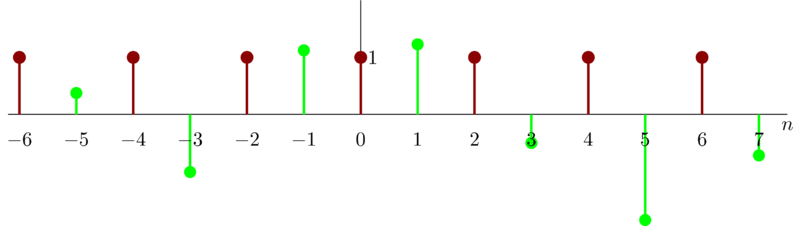
whose fundamental period is \(T_{0} = \frac{2\pi }{4\pi} = \frac{1}{2}\). Then the sampling interval \(T\) must satisfies that \(T/T_{0}\) is a rational number so that \(x[n]= x(nT)= \cos(4\pi nT )\) is a periodic signal.
Let \(T\), say, be \( \frac{1}{5} \), then
\begin{equation*} \frac{T}{T_{0}} = \frac{2}{5} \end{equation*}
The fundamental period of \(x[n]\) is \( N = \frac{q}{\mathrm{gcd}(p,q)} = \frac{5}{\mathrm{gcd}(2,5)} = 5 \).
We can visualize \(x(t)\) and \(x[n]\) as below.
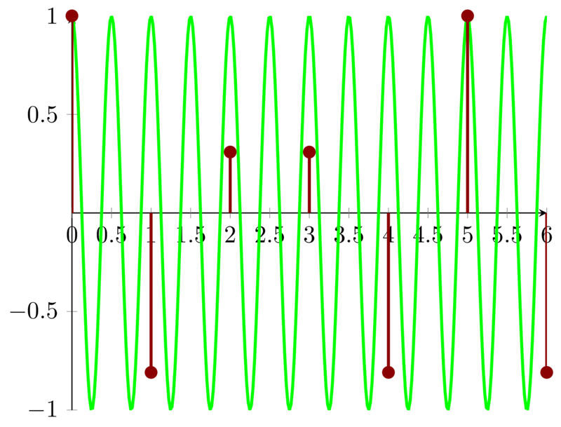
From the above figure, we can see that the discrete-time signal \(x[n]\) has fundamental period of \(5\) and its counterparts has fundamental period \(\frac{1}{2}\). We need at least \(10\) period of \(x(t)\) to get one period of \(x[n]\).
Now, if we take the Nyquist’s sampling into consideration, we must sampling a baseband signal with at least two times higher frequency of the signal to recover the baseband signal without alias. i.e. we must sample \(x(t) = \cos(4\pi t)\) with a signal of fundamental frequency \(8\pi\) to get signal \(x[n] = \cos(8\pi n)\).
6 Problem 1.37
An important concept in many communications applications in the correlation between two signals. In the problems at the end of Chapter 2, we will have more to say about this topic and will provide some indication of how it is used in practice. For now, we content ourselves with a brief introduction to correlation functions and some of their properties.
Let \(x(t)\) and \(y(t)\) be two signals; then the correlation function is defined as
\begin{equation*} \phi_{xy}(t) = \int_{-\infty}^{+\infty} x(t+ \tau) y(\tau)d\tau \end{equation*}
The function \(\phi_{xx}(t)\) is usually referred to as the autocorrelation function of the signal \(x(t)\) , while \(\phi_{xy}(t)\) is often called a cross-correlation function.
- What is the relationship between \(\phi_{xy}(t)\) and \(\phi_{yx}(t)\) ?
- Compute the odd part of \(\phi_{xx}(t)\).
- Suppose that \(y(t)= x(t+ T)\). Express \(\phi_{xy}(t)\) and \(\phi_{yy}(t)\) in terms of \(\phi_{xx}(t)\).
by the definition of correlation, we have
\begin{equation*} \phi_{yx} = \int_{-\infty}^{+\infty} y(t + \tau)x(\tau) d \tau \end{equation*}
we set \(t+ \tau = s\), then
\begin{eqnarray*}
\phi_{yx}(t) &=& \int_{-\infty}^{+\infty} y(t + \tau)x(\tau) d \tau \\
&=& \int_{-\infty}^{+\infty} x(s-t) y(s) ds \\
&=& \phi_{xy}(-t)
\end{eqnarray*}
Using the same procedure, we can also have \( \phi_{xy}(t) = \phi_{yx}(-t) \).
Problem 1.37b
we have
\begin{equation*} \phi_{xx}(t) = \int_{-\infty}^{+\infty} x(t+\tau)x(\tau) d\tau \end{equation*}
the odd part of \(\phi_{xx}(t)\) can be expressed as
\begin{equation*} \phi_{oxx}(t) = \frac{\phi_{xx}(t) - \phi_{xx}(-t)}{2} \end{equation*}
Based on Problem 1.37a, we have \( \phi_{xx}(t) = \phi_{xx}(-t) \) , so \(\phi_{oxx}(t) = 0\). which means that \(\phi_{oxx}(t)\) is an even signal.
Problem 1.37c
\begin{eqnarray*}
\phi_{xy}(t) &=& \int_{-\infty}^{+\infty} x(t+ \tau) y(\tau)d\tau \\
&=& \int_{-\infty}^{+\infty} x(t+ \tau) x(\tau + T)d\tau \\
&=& \int_{-\infty}^{+\infty} x(t + s -T) x(s) ds
\end{eqnarray*}
So we have \(\phi_{xy}(t) = \phi_{xx}(t-T)\).
\begin{eqnarray*}
\phi_{yy}(t) &=& \int_{-\infty}^{+\infty} y(t+ \tau) y(\tau)d\tau \\
&=& \int_{-\infty}^{+\infty} x(t+ \tau + T) x(\tau + T)d\tau \\
&=& \int_{-\infty}^{+\infty} x(t + s) x(s) ds
\end{eqnarray*}
So we have \(\phi_{yy}(t) = \phi_{xx}(t)\).
7 Problem 1.38
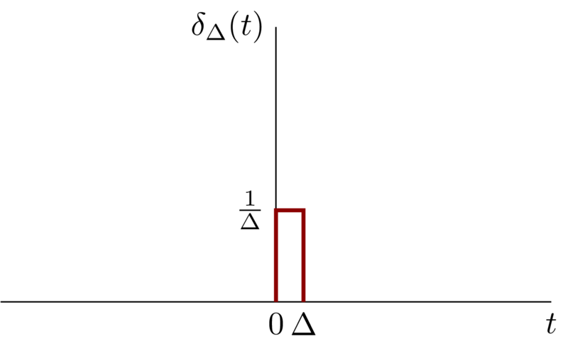
In this problem, we examine a few of the properties of the unit impulse function. a. show that
\begin{equation*} \delta(2t) = \frac{1}{2} \delta(t) \end{equation*}
Hint: Examine \(\delta_{\Delta}(t)\). (See Figure 1.34 in the textbook). b. In Section 1.4, we defined the continuous-time unit impulse as the limit of the signal \(\delta_{\Delta}(t)\). More precisely, we defined several of the properties of \(\delta(t)\) by examining the corresponding properties of \(\delta_{\Delta}(t)\). For example, since the signal
\begin{equation*} u_{\Delta}(t) = \int_{-\infty}^{t}\delta_{\Delta}(\tau)d\tau \end{equation*}
converges to the unit step:
\begin{equation*} u(t) = \lim_{\Delta\to 0} u_{\Delta}(t), \end{equation*}
we could interpret \(\delta(t)\) through the equation
\begin{equation} \label{eq:problem1-38-1} u(t) = \int_{-\infty}^{t} \delta(\tau)d\tau \end{equation}
or by viewing \(\delta(t)\) as the formal derivative of \(u(t)\).
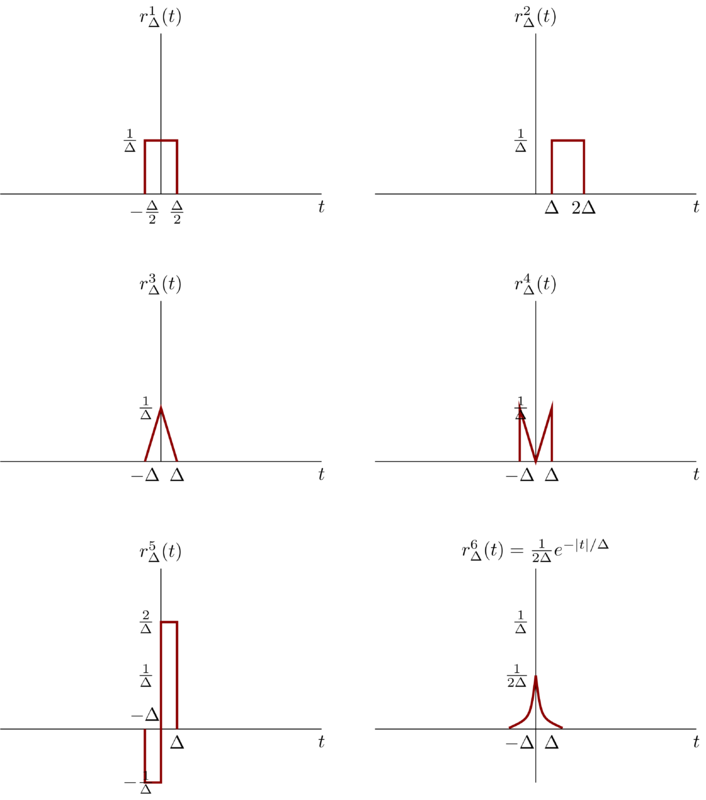
This type of discussion is important, as we are in effect trying to define \(\delta(t)\) through its properties rather than by specifying its value for each \(t\), which is not possible. In Chapter 2, we provide a very simple characterization of the behavior of the unit impulse that is extremely useful in the study of linear time-invariant systems. For the present, however, we concentrate on demonstrating that the important concept in using the unit impulse is to understand how it behave. To do this, consider the six signals depicted in Figure shown below. Show that each “behaves like an impulse” as \(\Delta\to 0\) in that, if we let
\begin{equation*} u_{\Delta}^{i}(t) = \int_{-\infty}^{t} r_{\Delta}^{i}(\tau)d\tau, \end{equation*}
then
\begin{equation*} \lim_{\Delta\to 0} u_{\Delta}^{i}(t) = u(t) \end{equation*}
In each case, sketch and label carefully the signal \(u_{\Delta}^{i}(t)\). Note that
\begin{equation*} r_{\Delta}^{2}(0) = r_{\Delta}^{4}(0) = 0 \ \forall \Delta \end{equation*}
Therefore, it is not enough to define or to think of \(\delta(t)\) as being zero for \(t\neq 0\) and infinite for \(t=0\). Rather, it is properties such as equation (\ref{eq:problem1-38-1}) that define the impulse. In Section 2.5 we will define a whole class of signals known as singularity function, which are related to the unit impulse and which are also defined in terms of their properties rather than their values.
Problem 1.38a
Base on fig 1 , \(\delta(2t)\) can be visualized as follows
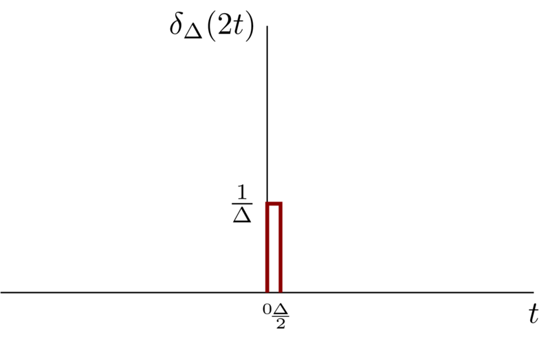
Based on the fact \(\delta(t)\) has unit area, so \(\delta(2t)\) will have \(\frac{1}{2}\) . So \(\delta(2t) = \frac{1}{2}\delta(t)\).
Problem 1.38b
Because
\begin{equation*} u_{\Delta}(t) = \int_{-\infty}^{t}\delta_{\Delta}(\tau)d\tau \end{equation*}
We can get \(u_{\Delta}^{1}(t)\) easily.
\(r_{\Delta}^{1}(t)\) can be represented as
\begin{equation*}
r_{\Delta}^{1}(t) =
\begin{cases}
\frac{1}{\Delta}, & -\frac{\Delta}{2} \leq t \leq \frac{\Delta}{2} \\
0, & \mathrm{Otherwise}
\end{cases}
\end{equation*}
Then during the integration, \(u_{\Delta}^{1}(t)\) can be represented as
\begin{equation*}
u_{\Delta}^{1}(t) =
\begin{cases}
0, & t < -\frac{\Delta}{2} \\
\frac{t}{\Delta}, & -\frac{\Delta}{2} \leq t \leq \frac{\Delta}{2} \\
1, & t > \frac{\Delta}{2}
\end{cases}
\end{equation*}

we can express the \(r_{\Delta}^{2}(t)\) as :
\begin{equation*}
r_{\Delta}^{2}(t) =
\begin{cases}
\frac{1}{\Delta} , & \Delta \leq t \leq 2\Delta \\
0, & \mathrm{Otherwise}
\end{cases}
\end{equation*}
So the \(u_{\Delta}^{2}(t)\) can be expressed as:
\begin{equation*}
u_{\Delta}^{2}(t) =
\begin{cases}
0, & t < \Delta \\
\frac{t-\Delta}{\Delta} & \Delta \leq t \leq 2\Delta \\
1, & t> 2\Delta
\end{cases}
\end{equation*}

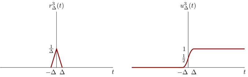
We express \(r_{\Delta}^{3}(t)\) as:
\begin{equation*}
r_{\Delta}^{3}(t) =
\begin{cases}
\frac{1}{\Delta^{2}} ( t + \Delta) , & - \Delta < t \leq 0 \\
\frac{1}{\Delta^{2}} ( -t + \Delta) , & 0 < t \leq \Delta \\
0, & \mathrm{otherwise}
\end{cases}
\end{equation*}
and \(u_{\Delta}^{3}(t)\):
\begin{equation*}
u_{\Delta}^{3}(t) =
\begin{cases}
\frac{1}{\Delta^{2}}( \frac{t^{2}}{2} + \Delta t + \frac{\Delta^{2}}{2}) ,& -\Delta < t \leq 0 \\
\frac{1}{2} + \frac{1}{\Delta^{2}} ( - \frac{t^{2}}{2} + \Delta t ) , & 0 < t < \Delta \\
1, & t > \Delta
\end{cases}
\end{equation*}
So we can visualize them as follows:
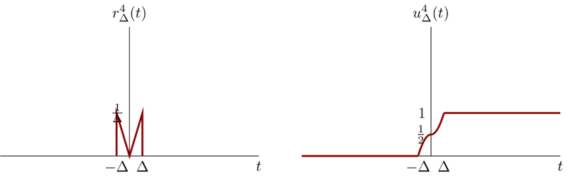
We can represent \(r_{\Delta}^{4}(t)\) as :
\begin{equation*}
r_{\Delta}^{4}(t) =
\begin{cases}
- \frac{1}{\Delta^{2}} t , & -\Delta < t \leq 0 \\
\frac{1}{\Delta^{2}} t , & 0 < t \leq \Delta \\
0, & \mathrm{Otherwise}
\end{cases}
\end{equation*}
and \(u_{\Delta}^{4}(t)\)
\begin{equation*}
u_{\Delta}^{4}(t) =
\begin{cases}
0, & t < -\Delta \\
- \frac{t^{2}}{2\Delta^{2}} + \frac{1}{2}, & - \Delta < t \leq 0\\
\frac{t^{2}}{2\Delta^{2}} + \frac{1}{2}, & - \Delta < t \leq 0\\
1, & t > \Delta
\end{cases}
\end{equation*}
and we visualize them as:
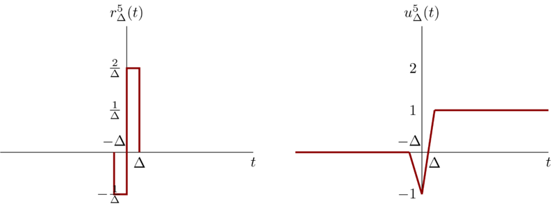
We can express \(r_{\Delta}^{5}(t)\) as :
\begin{equation*}
r_{\Delta}^{5}(t) =
\begin{cases}
- \frac{1}{\Delta} , & -\Delta < t \leq 0 \\
\frac{2}{\Delta} , & 0 < t \leq \Delta \\
0, & \mathrm{Otherwise}
\end{cases}
\end{equation*}
and \(u_{\Delta}^{5}(t)\) as:
\begin{equation*}
u_{\Delta}^{5}(t) =
\begin{cases}
- \frac{t}{\Delta} -1, & -\Delta < t < 0 \\
-1 + \frac{2t}{\Delta} , & 0 < t \leq \Delta \\
1,& t > \Delta
\end{cases}
\end{equation*}
So we can visualize them as below:
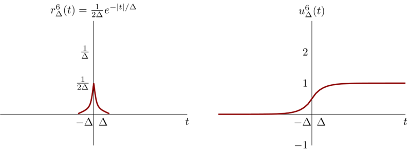
We can express \(r_{\Delta}^{6}(t)\) as :
\begin{equation*} r_{\Delta}^{6}(t) = \frac{1}{2\Delta} e^{-|t|/\Delta} \end{equation*}
and \(u_{\Delta}^{6}(t)\) as :
\begin{equation*}
u_{\Delta}^{6}(t) =
\begin{cases}
\frac{1}{2} e^{\frac{t}{\Delta}} , & t< 0 \\
1 - \frac{1}{2}e^{ \frac{-t}{\Delta}} , & t> 0 \\
\end{cases}
\end{equation*}
So we can visualize them as below:
8 Problem 1.39
The role played by \(u(t)\) and \(\sigma(t)\) and other singularity functions in the study of linear time-invariant systems is that of an idealization of a physical phenomenon, and, as we will see, the use of these idealizations allow us to obtain an exceedingly important and very simple representation of such systems. In using singularity functions, we need, however, to be careful. In particular, we must remember that they are idealizations, and thus, whenever we perform a calculation using them, we are implicitly assuming that this calculation represents an accurate description of the behavior of the signals that they are intended to idealize. To illustrate, consider the equation
\begin{equation} \label{eq:prob1-39-0} x(t)\sigma(t) = x(0)\sigma(t) \end{equation}
This equation is based on the observation that
\begin{equation} \label{eq:prob1-39-1} x(t)\sigma_{\Delta}(t) \approx x(0)\sigma_{\Delta}(t) \end{equation}
Taking the limit of this relationship then yields the idealized one given by equation (\ref{eq:prob1-39-0}). However, a more careful examination of our derivation of equation (\ref{eq:prob1-39-1}) shows that that equation really makes senses only if \(x(t)\) is continuous at \(t=0\). If it is not, then we will not have \(x(t)\approx x(0)\) for \(t\) small.
To make this point clearer, consider the unit step signal \(u(t)\). Recall from the following equation:
\begin{equation*}
u(t) =
\begin{cases}
0, & t< 0\\
1, & t> 0
\end{cases}
\end{equation*}
that
- \(u(t)= 0\) for \(t<0\)
- \(u(t) = 1\) for \(t> 0\),
but that its value at \(t=0\) is not defined. The fact that \(u(0)\) is not defined is not particularly bothersome, as long as the calculations we perform using \(u(t)\) do not rely on a specific choice for \(u(0)\). For example, if \(f(t)\) is a signal that is continuous at \(t=0\), then the value of
\begin{equation*} \int_{-\infty}^{+\infty} f(\sigma) u(\sigma) d \sigma \end{equation*}
does not depend upon a choice for \(u(0)\). On the other hand, the fact that \(u(0)\) is undefined is significant in that it means that certain calculations involving singularity functions are undefined. Consider trying to define a value for the product \(u(t)\delta(t)\).
To see that this cannot be defined, show that
\begin{equation*} \lim_{\Delta\to 0} [u_{\Delta}(t)\delta(t)] = 0, \end{equation*}
but
\begin{equation*} \lim_{\Delta\to 0} [u_{\Delta}(t)\delta_{\Delta}(t)] = \frac{1}{2} \delta(t) \end{equation*}
In general, we can define the product of two signals without any difficulty, as long as the signals do not contain singularities ( discontinuities, impulse, or the other singularities introduced in Section 2.5) whose locations coincide. When the locations do coincide, the product is undefined. As an example, show that the signal
\begin{equation*} g(t) = \int_{-\infty}^{+\infty} u( \tau )\delta(t-\tau)d\tau \end{equation*}
is identical to \(u(t)\); that is, it is \(0\) for \(t < 0\), it equals \(1\) for \(t> 0\), and it is undefined for \(t=0\)
\begin{equation*} \lim_{\Delta\to 0} [u_{\Delta}(t)\delta(t)] = \lim_{\Delta\to 0} [u_{\Delta}(t)\delta(0)] = 0 \end{equation*}
And
\begin{eqnarray*}
\lim_{\Delta\to 0} [u_{\Delta}(t)\delta_{\Delta}(t)] &=& \lim_{\Delta\to 0 } \frac{1}{2} \frac{d u_{\Delta}^{2}(t)}{dt} \\
&=& \frac{1}{2} \delta(t)
\end{eqnarray*}
Notice that when \(\Delta\to 0\) the item \( \frac{u_{\Delta}^{2}(t)}{dt} \) also approach to \(\delta(t)\).
for equation:
\begin{equation*} g(t) = \int_{-\infty}^{+\infty} u( \tau )\delta(t-\tau)d\tau \end{equation*}
we have
\begin{equation*}
g(t) =
\begin{cases}
0, & t< 0 \\
1, & t> 0 \\
\mathrm{undefined}, & t = 0
\end{cases}
\end{equation*}
So \(g(t)\) has the same property as \(u(t)\)
9 Problem 1.40
- Show that if a system is either additive or homogeneous, it has the property that if the input is identically zero, then the output is also identically zero.
- Determine a system (either in continuous or discrete time) that is neither additive nor homogeneous but which has a zero output if the input is identically zero.
- From part (a) can you include that if the input to a linear system is zero between times \(t_{1}\) and \(t_{2}\) in continuous time or between times \(n_{1}\) and \(n_{2}\) in descrete time, then its output must also be zero between these same times? Explain your answer.
Problem 1.40a
Let \(x_{1}(t)\) and \(x_{2}(t)\) be two input signals of system \(\mathcal{S}\), and \(y_{1}(t)\) and \(y_{2}(t)\) two output respectively. The system is represented as \(y(t) = f(x(t))\). Then
\begin{eqnarray*}
y_{1}(t)&=& f(x_{1}(t)) \\
y_{2}(t)&=& f(x_{2}(t))
\end{eqnarray*}
Let \(x_{3}(t)= x_{1}(t) + x_{2}(t)\), then by the definition of additive property
\begin{equation*} y_{3}(t) = f(x_{3}(t)) = f(x_{1}(t) + x_{2}(t)) = y_{1}(t) + y_{2}(t) \end{equation*}
If \(x_{1}(t)= x_{2}(t) = 0\) , then \(x_{3}(t) = 0\) and we have
\begin{equation*} f(0) = 2f(0) \end{equation*}
So, \(f(0) = 0\). i.e. If a system is additive and the input is identically zero, then the output is also identically zero.
Next we show that if a system is homogeneous, the property also holds.
Let \(x_{1}(t)\) be input signals of system \(\mathcal{S}\), and \(x_{2}(t)= \alpha x_{1}(t)\) another input. we have \(y_{1}(t) = f(x_{1}(t))\) and \(y_{2}(t) = f(x_{2}(t)) = \alpha f(x_{1}(t))\). If \(x_{1}(t) = 0 \), then \(x_{2}(t) = 0\) so \(y_{2}(t) = f(0) = \alpha f(0)\). Then we have \(f(0) = 0 = y_{2}(t)\). i.e. if a system is homogeneous and the input is identically zero, then the output is also identically zero.
Problem 1.40b
It is easy to construct such a system, for a continuous-time version, we have \(y(t) = x^{2}(t)\) and it discrete-time counterparts \(y[n] = x^{2}[n]\)
We cannot reach that conclusion. Because for a system has memory, a certain zero period \(t_{1}\) to \(t_{2}\) does not result the same zero period in the output. Let’s take \(y[n] = x[n-n_{0}]\) where \(n_{0}\neq 0\), the output will have a delay ( \(n_{0}\) is positive) and an advance ( \(n_{0}\) is negative).
10 Problem 1.41
Consider a system \(\mathcal{S}\) with input \(x[n]\) and output \(y[n]\) related by
\begin{equation*} y[n] = x[n]\{ g[n] + g[n-1] \} \end{equation*}
- If \(g[n] = 1\) for all \(n\), show that \(S\) is time invariant.
- If \(g[n] = n\) , show that \(\mathcal{S}\) is not time invariant.
- If \(g[n] = 1 + (-1)^{n}\), show that \(\mathcal{S}\) is time invariant.
Problem 1.41a
If \(g[n] = 1 \forall \ n\) , then we have
\begin{equation*} y[n] = 2x[n] \end{equation*}
Next, we proof that this system is time invariant. Let \(x_{1}[n]\) and \(y_{1}[n]\) are the input and output respectively i.e.
\begin{equation*} y_{1}[n] = 2x_{1}[n] \end{equation*}
Let \(x_{2}[n] = x_{1}[n-n_{0}]\) then we have
\begin{equation*} y_{2}[n] = 2x_{2}[n] = 2x_{1}[n-n_{0}] = 2y_{1}[n-n_{0}] \end{equation*}
So we have that one time shift in the input signal will result in an identical time shift in the output. The system is time invariant.
if \(g[n] = n\), we have
\begin{equation*} y[n] = (2n-1) x[n] \end{equation*}
Let \(x_{1}[n]\) and \(y_{1}[n]\) the input and output respectively, i.e.
\begin{equation*} y_{1}[n] = (2n-1)x_{1}[n] \end{equation*}
Let \(x_{2}[n] = x_{1}[n-n_{0}]\), then we have
\begin{equation*} y_{2}[n] = (2n-1)x_{2}[n] = (2n-1)x_{1}[n-n_{0}] \end{equation*}
We also have:
\begin{equation*} y_{1}[n-n_{0}] = ( 2(n-n_{0}) ) x_{1}[n-n_{0}] \end{equation*}
Obviously, \(y_{2}[n]\neq y_{1}[n-n_{0}]\). The system is time invariant.
If \(g[n] = 1 + (-1)^{n}\), then
\begin{equation*} g[n] + g[n-1] = 1 + (-1)^{n} + 1 + (-1)^{n-1} = 2 \end{equation*}
Which means that the system is identical as the system in part (a) and hence the system is time invariant.
11 Problem 1.42
Is the following statement true or false?
The series interconnection of two linear time-invariant system is itself a linear, time-invariant system.
Justify your answer.
Is the following statement true or false?
The series interconnection of two nonlinear systems is itself nonlinear.
Justify your answer.
Consider three systems with the following input-output relationships:
System 1:
\begin{equation*} y[n] = \begin{cases} x[n/2], & n\ \mathrm{even} \\
0, & n\ \mathrm{odd} \end{cases} \end{equation*}System 2:
\begin{equation*} y[n] = x[n] + \frac{1}{2}x[n-1] + \frac{1}{4}x[n-2] \end{equation*}
System 3:
\begin{equation*} y[n] = x[2n] \end{equation*}
Suppose that these systems are connected in series as depicted in Figure below. Find the input-output relationship for the overall interconnected system. Is this system linear? Is it time invariant?

Let \(\mathcal{S}_{1}\) and \(\mathcal{S}_{2}\) two connected LTI system. Let \(x_{11}(t)\) and \(x_{12}(t)\) arbitrary signals, \(a_{1}\) and \(b_{1}\) arbitrary consstants.
Then:
\begin{eqnarray*}
x_{11}(t)&\xrightarrow{\mathcal{S}_{1}} & y_{11}(t) \\
x_{12}(t)&\xrightarrow{\mathcal{S}_{1}} & y_{12}(t) \\
\end{eqnarray*}
Let \(x_{13}(t) = a_{1} x_{11}(t) + b_{1}x_{12}(t)\), then
\begin{equation*} x_{13}(t) = a_{1} x_{11}(t) + b_{1}x_{12}(t) \xrightarrow{\mathcal{S}_{1}} y_{13}(t) = a_{1}y_{11}(t) + b_{1} y_{12}(t) \end{equation*}
For System \(\mathcal{S}_{2}\), we have the similar results:
\begin{eqnarray*}
x_{21}(t)&\xrightarrow{\mathcal{S}_{2}} & y_{21}(t) \\
x_{22}(t)&\xrightarrow{\mathcal{S}_{2}} & y_{22}(t) \\
\end{eqnarray*}
Let \(x_{23}(t) = a_{2} x_{21}(t) + b_{2}x_{22}(t)\), then
\begin{equation*} x_{23}(t) = a_{2} x_{21}(t) + b_{2}x_{22}(t) \xrightarrow{\mathcal{S}_{2}} y_{23}(t) = a_{2}y_{21}(t) + b_{2} y_{22}(t) \end{equation*}
Because \(S_{1}\) and \(S_{2}\) are interconnected in series. So let \( x_{21}(t) = y_{11}(t) \) and \(x_{22}(t) = y_{12}(t)\) we can see the overall system is linear.
Next we check the time invariant property of the overall system. Since \(\mathcal{S}_{1}\) and \(S_{2}\) are time invariant. we have
\begin{eqnarray*}
x_{1}(t-t_{1})&\xrightarrow{\mathcal{S}_{1}}& y_{1}(t-t_{1}) \\
x_{2}(t-t_{2})&\xrightarrow{\mathcal{S}_{2}}& y_{2}(t-t_{2})
\end{eqnarray*}
Since the two systems are in series, the overall system is time invariant.
False, we just take one counterexample. Consider the following two nonlinear systems.
\begin{eqnarray*}
y_{1}[n] &=& x_{1}[n] + 1 \\
y_{2}[n] &=& x_{2}[n] - 1
\end{eqnarray*}
Since the two systems are in series. Let \(y_{1}[n] = x_{2}[n]\), then we have the overall system \(y_{2}[n] = x_{1}[n]\) which is linear.
First we can express the interconnection of system 1 and system 2 as:
\begin{equation*}
y[n] =
\begin{cases}
x[ \frac{n}{2} ] + \frac{1}{4} x[ \frac{n-2}{2} ] , & n \ \mathrm{even} \\
\frac{1}{2} x[ \frac{n-1}{2} ] , & n \ \mathrm{odd}
\end{cases}
\end{equation*}
Then we express the interconnection of all the three systems.
\begin{equation*} y[n] = x[ \tfrac{2n}{2} ] + \tfrac{1}{4} x[ \tfrac{2n-2}{2} ] = x[n] + \tfrac{1}{4} x[n-1] \end{equation*}
So the system is an LTI system.
12 Problem 1.43
- Consider a time-invariant system with input \(x(t)\) and output \(y(t)\). Show that if \(x(t)\) is periodic with period \(T\), then so is \(y(t)\). Show that the analogous result also holds in descrete time.
- Give an example of a time-invariant system and a nonperiodic input signal \(x(t)\) such that the corresponding output \(y(t)\) is periodic.
Problem 1.43a
For a time-invariant system, an arbitrary time shifting \(t_{0}\) in the input will result in an identical time shifting in the output. So let the \(t_{0}\) be the period \(T\), the the output should also be a time shifting \(T\). Because the system is period \(x(t) = x(t+T)\), then the output \(y(t) = y(t+T)\).
For the descrete time, the conclusion also holds.
Suppose that we have a system:
\begin{equation*} y[n] = 1 \end{equation*}
Then this system is time-invariant, any input will not change the property of its output.
13 Problem 1.44
Show that causality for a continuous-time linear system is equivalent to the following statement:
For any time \(t_{0}\) and any input \(x(t)\) such that \(x(t) = 0\) for \(t<t_{0}\), the corresponding output \(y(t)\) must also be zero for \(t< t_{0}\).
The analogous statement can be made for a discrete-time linear system.
Find a nonlinear system that satisfies the foregoing condition but is not causal.
Find a nonlinear system that is causal but does not satisfy the condition.
Show that invertibility for a discrete-time linear system is equivalent to be the following statement:
The only input that produces \(y[n] = 0 \) for all \(n\) is \(x[n]= 0\) for all \(n\).
The analogous statement is also true for a continuous-time linear system.
Find a nonlinear system that satisfies the condition of part (d) but is not invertible.
Problem 1.44a
A system is causal if the output at any time depends on values of the input at only the present and past times.
Let’s suppose that \(y(t) \neq 0, t< t_{0} \), which mean for some \(x(t) \neq 0, t< t_{0}\). However this is not true. So for \(x(t) = 0, t< t_{0}\), it must be that \(y(t)= 0 , t< t_{0}\)
\(y(t) = x^{2}(t)x^{2}(t+1)\) where \(x(t) = 0, t< t_{0}\).
\(y(t) = x(t) + 1\)
First let’s proof that suppose \(y[n] = 0, \forall n\) if \(x[n]=0 ,\forall n\) , then the system is invertible.
let \(x_{1}[n]\) and \(x_{2}[n]\) be two arbitrary inputs and these two inputs lead to the same output \(y_{1}[n]\) .
\begin{eqnarray*}
x_{1}[n] &\xrightarrow{\mathcal{S}}& y_{1}[n] \\
x_{2}[n] &\xrightarrow{\mathcal{S}}& y_{1}[n]
\end{eqnarray*}
Because the system is linear.
\begin{equation*} x_{1}[n] - x_{2}[n] \xrightarrow{\mathcal{S}} y_{1}[n]-y_{1}[n] = 0 \end{equation*}
So we must have \(x_{1}[n] = x_{2}[n]\) which is not consist with the assumption and means that any output \(y_{1}[n]\) must have single one input. i.e. the system is invertible.
Next we proof that for a invertible linear system, \(y[n] = 0, \forall n \) if and only if \(x[n] = 0, \forall n\)
If \(x[n] = 0\), then we have
\begin{eqnarray*}
x[n] = 0 &\xrightarrow{\mathcal{S}} &y[n] \\
\alpha x[n] = 0 &\xrightarrow{\mathcal{S}}& \alpha y[n]
\end{eqnarray*}
where \(\alpha\) is arbitrary constants. Because the system is invertible, so the same input \(0\) must lead to the same output, so \(y[n]=\alpha y[n] \). then \(y[n] = 0\).
\(y[n] = x^{m}[n] , m\neq 1 \ \mathrm{and}\ m\neq 0 \)
\(m=1\) \(y[n] = x[n]\) is a linear system. \(m=0\), \(y[n] = 1\) does satisfies that \(y[n]= 0, \forall n\)
14 Problem 1.45
In Problem 1.37, we introduced the concept of correlation functions. It is often important in practice to compute the correlation function \(\phi_{hx}(t)\) where \(h(t)\) is a fixed given signal, but where \(x(t)\) may be any of a wide variety of signals. In this case, what is done is to design a system \(\mathcal{S}\) with input \(x(t)\) and output \(\phi_{hx}(t)\).
- Is \(\mathcal{S}\) linear ? Is \(\mathcal{S}\) time invariant? Is \(\mathcal{S}\) causal? Explain your answers.
- Do any of your answers to part (a) change if we take as the output \(\phi_{xh}(t)\) rather than \(\phi_{hx}(t)\)?
First, let’s recall the definition of \(\phi_{hx}(t)\):
\begin{equation*} \phi_{hx}(t) = \int_{-\infty}^{+\infty} h(t + \tau)x(\tau)d\tau \end{equation*}
Problem 1.37a
Let \(x_{1}(t)\) and \(x_{2}(t)\) two arbitrary input signals, and \(\alpha\) and \(\beta\) two arbitrary constants. Let \(x_{3}(t) = \alpha x_{1}(t) + \beta x_{2}(t) \), then we have
\begin{eqnarray*}
\phi_{hx_{1}}(t) &=& \int_{-\infty}^{+\infty} h(t+\tau)x_{1}(\tau)d\tau \\
\phi_{hx_{2}}(t) &=& \int_{-\infty}^{+\infty} h(t+\tau)x_{2}(\tau)d\tau \\
\phi_{hx_{3}}(t) &=& \int_{-\infty}^{+\infty} h(t+\tau)x_{3}(\tau)d\tau \\
&=& \int_{-\infty}^{+\infty} h(t+\tau)( \alpha x_{1}(t) + \beta x_{2}(t) )d\tau \\
&=& \alpha \int_{-\infty}^{+\infty} h(t+\tau)x_{1}(\tau)d\tau + \beta \int_{-\infty}^{+\infty} h(t+\tau)x_{2}(\tau)d\tau \\
&=& \alpha \phi_{hx_{1}}(t) + \beta \phi_{hx_{2}}(t)
\end{eqnarray*}
Then we have that the system is linear.
Next we check the property of time invariance.
Let \(x_{4}(t) = x_{1}(t+T_{0})\) So
\begin{eqnarray*}
\phi_{hx_{4}}(t) &=& \int_{-\infty}^{+\infty} h(t+\tau)x_{4}(\tau)d\tau \\
&=& \int_{-\infty}^{+\infty} h(t+\tau)x_{1}(\tau + T_{0})d\tau \\
&=& \int_{-\infty}^{+\infty} h(t+s-T_{0})x_{1}(s)ds \\
&=& \phi_{hx_{1}}(t-T_{0})
\end{eqnarray*}
We have \(\phi_{hx_{4}}(t)\neq \phi_{hx_{1}}(t+T_{0})\). So the system is not time invariant.
The system is not causal, because the output depends on all time of the input.
\(\phi_{xh}(t)\) can be expressed as
\begin{equation*} \phi_{xh}(t) = \int_{-\infty}^{+\infty} x(t+ \tau) h(\tau)d\tau \end{equation*}
Based on similar analysis as in part (a), we can conclude that the system is linear.
Next, we check the property of time invariance. Let \(x_{1}(t)\) be arbitrary input signal and \(x_{4}(t) = x_{1}(t+T_{0})\) then we have
\begin{eqnarray*}
\phi_{x_{4}h}(t) &=& \int_{-\infty}^{+\infty} x_{4}(t+\tau) h(\tau) d\tau \\
&=& \int_{-\infty}^{+\infty} x_{1}(t+T_{0}+\tau) h(\tau) d\tau \\
&=& \phi_{x_{1}h}(t+T_{0}) = \phi_{x_{1}h}(t+T_{0})
\end{eqnarray*}
Which means that the system is time invariant.
The system is not causal because the output depends on all the value of \(x(t)\).
15 Problem 1.46
Consider the feedback system of Figure shown as below. Assume that \(y[n] = 0, n<0\)
- Sketch the output when \(x[n] = \delta[n]\)
- Sketch the output when \(x[n] = u[n]\)
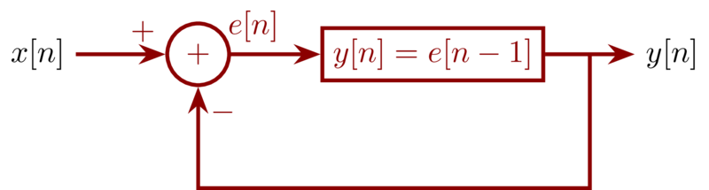
From the figure given, we have:
\begin{eqnarray*}
e[n]&=& x[n] - y[n] \\
y[n] &=& e[n-1]
\end{eqnarray*}
So we have \(y[n] = x[n-1] - y[n-1]\)
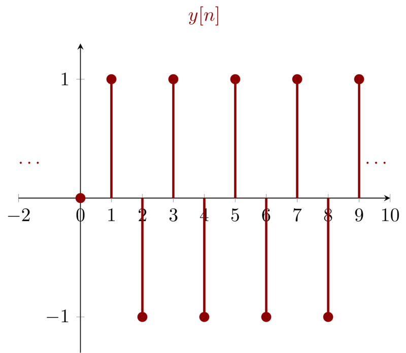
Problem 1.46a
\(x[n] = \sigma[n]\) So we have \(x[0] = 1\) and \(x[n] = 0, n\neq 0\)
\begin{eqnarray*}
y[0]&=& x[-1] - y[-1] = 0 \\
y[1]&=& x[0] - y[0] = 1 \\
y[2]&=& x[1] - y[1] = -1 \\
y[3]&=& x[2] - y[2] = 1 \\
\end{eqnarray*}
So the output can be sketched as:
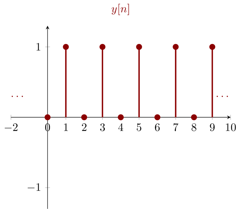
Problem 1.46b
\(x[n] = u[n]\) So we have \(x[n] = 1, n\geq 0\)
\begin{eqnarray*}
y[0]&=& x[-1] - y[-1] = 0 \\
y[1]&=& x[0] - y[0] = 1 \\
y[2]&=& x[1] - y[1] = 0 \\
y[3]&=& x[2] - y[2] = 1 \\
\end{eqnarray*}
So the output can be sketched as:
16 Problem 1.47
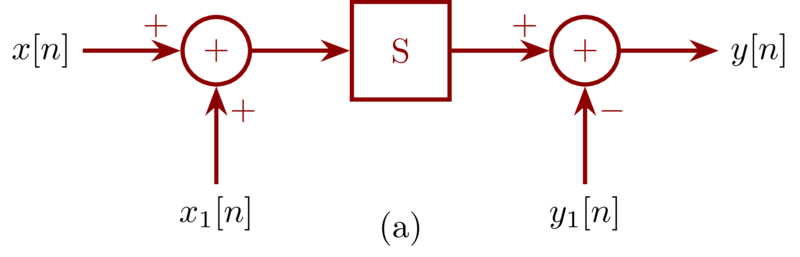
- Let \(\mathcal{S}\) denote an incrementally linear system, and let \(x_{1}[n]\) be an arbitrary input signal to \(\mathcal{S}\) with corresponding output \(y_{1}[n]\). Consider the system illustrated in Figure 1-47(a). Show that this system is linear and that, in fact, the overall input-output relationship between \(x[n]\) and \(y[n]\) does not depend on the particular choice of \(x_{1}[n]\).
- Use the result of part (a) to show that \(\mathcal{S}\) can be represented in the form shown in Figure 1-48 .
Which of the following systems are incrementally linear? Justify your answers, and if a system is incrementally linear, identify the linear system \(L\) and the zero-input response \(y_{0}[n]\) or \(y_{0}(t)\) for the representation of the system as shown in Figure 1.48
- \(y[n] = n + x[n] + 2x[n+4]\)
The system is shown as below
\begin{equation*} y[n] = \begin{cases} n/2, & n\ \mathrm{even}\\
(n-1)/2 + \sum_{k=-\infty}^{(n-1)/2} x[k],& n\ \mathrm{odd} \end{cases} \end{equation*}The system is shown as below
\begin{equation*} y[n] = \begin{cases} x[n] - x[n-1] + 3, & \mathrm{if}\ x[0] \geq 0 \\
x[n] - x[n-1] - 3, & \mathrm{if}\ x[0] < 0 \end{cases} \end{equation*}The system depicted in Figure 1-47(b)
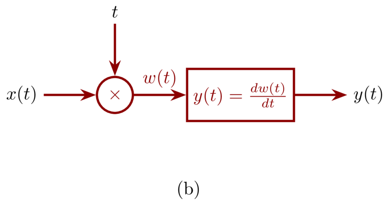
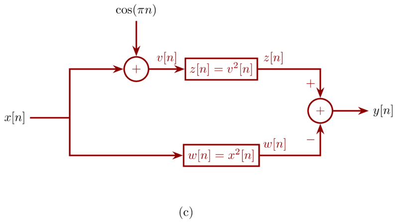
The system depicted in Figure 1-47©
Suppose that a particular incrementaly linear system has a representation as in figure 1-48, with \(\mathcal{L}\) denoting the linear system and \(y_{0}[n]\) the zero input reponse, Show that \(S\) is time invariant if and only if \(\mathcal{L}\) is a time-invariant system and \(y_{0}[n]\) is constant.
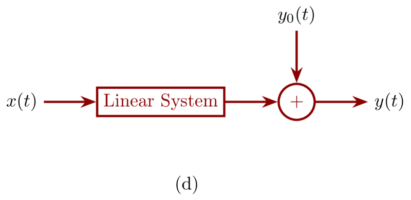
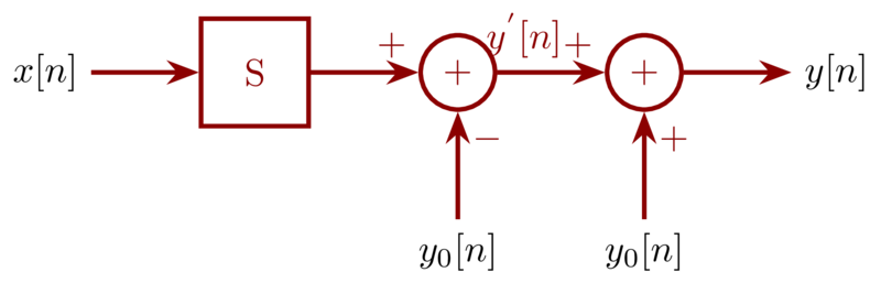
Problem 1.47a
An incrementally linear system can be expressed as Figure 1-47d : a linear system followed by another signal equal to the zero-input response of the system. Because \(\mathcal{S}\) is an incrementally linear system, the output \(y[n] = y^{‘}[n] - y_{1}[n]\) where \(y^{‘}[n]\) is the output of \(\mathcal{S}\). The \(y^{‘}[n]\) contains the response of \(x[n]\) and \(x_{1}[n]\) i.e. \(y^{‘}[n]\) at lease contains \(y_{1}[n]\). So \(y[n] = y^{‘}[n] - y_{1}[n]\) will not containt the zero-input response of system \(\mathcal{S}\). and the overall system from \(x[n]\) to \(y[n]\) only have the result of the linear part of system \(\mathcal{S}\) hence the system is linear.
Furthermore, no matter what \(x_{1}[n]\) we choose, its effect will be cancelled by substracting \(y_{1}[n]\). hence, the overall input-output relationship between \(x[n]\) and \(y[n]\) does not depend on the particular choice of \(x_{1}[n]\).
Problem 1.47b
\(\mathcal{S}\) is an incrementally linear system. By substracting its zero-input response \(y_{0}[n]\) we have a linear system.
The system from \(x[n]\) to \(y^{‘}[n]\) is the linear part, and the overall input-output is the system \(\mathcal{S}\) represented as incrementally linear system.
Problem 1.47c-1
The system is incrementally linear with the linear part:
\begin{equation*} x[n] \xrightarrow{\mathcal{L}} x[n] + 2x[n+4] \end{equation*}
and the zero-input response
\begin{equation*} y_{0}[n] = n \end{equation*}
Problem 1.47c-2
The system is incrementally linear with the linear part:
\begin{equation*}
x[n] \xrightarrow{\mathcal{L}}
\begin{cases}
0, & n\ \mathrm{even} \\
\sum_{k=-\infty}^{(n-1)/2}x[k], & n\ \mathrm{odd}
\end{cases}
\end{equation*}
and the zero-input response
\begin{equation*}
y_{0}[n] =
\begin{cases}
n/2 , & n\ \mathrm{even} \\
(n-1)/2, & n\ \mathrm{odd}
\end{cases}
\end{equation*}
Problem 1.47c-3
Not incrementally linear system. because for \(x[0] \geq 0\) there is one zero-input response \(+3\), for \(x[0] < 0\), there is one zero-input response \(-3\). So the overall system cannot choose one zero-input response.
Problem 1.47c-4
The overall system can be expressed as
\begin{equation*} y(t) = x(t) + t\frac{dx(t)}{t} \end{equation*}
The system is linear itself and of course is incrementally linear with zero-input reponse zero.
Problem 1.47c-5
The overall system can be expressed as:
\begin{eqnarray*}
y[n]&=& (x[n] + \cos(\pi n))^{2} - (x^{2}[n]) \\
&=& 2x[n]\cos(\pi n) + \cos^{2}(\pi n)
\end{eqnarray*}
Therefore, the system is incrementally linear with the linear part:
\begin{equation*} x[n] \xrightarrow{\mathcal{L}} 2x[n]\cos(\pi n) \end{equation*}
and the zero-input response
\begin{equation*} y_{0}[n] = \cos^{2}(\pi n) \end{equation*}
Problem 1.47d
First, let’s proof that if \(\mathcal{S}\) is time invariant we can conclude that \(\mathcal{L}\) is a time-invariant system and \(y_{0}[n]\) is constant
For the linear part we have:
\begin{equation*} x[n] \xrightarrow{\mathcal{L}} L[n] \end{equation*}
And the zero-input part.
\begin{equation*} y[n] = L[n] + y_{0}[n] \end{equation*}
Suppose \(\mathcal{S}\) is time invariant, let \(x_{1}[n]\) and arbitrary input signal.
\begin{equation*} y_{1}[n] = x_{1}[n] + y_{0}[n] \end{equation*}
and let \(x_{2}[n]\) be \(x_{1}[n-n_{0}]\), where \(n_{0}\) is an arbitrary integer So
\begin{equation*} y_{2}[n] = x_{2}[n] + y_{0}[n] = x_{1}[n-n_{0}] + y_{0}[n] \end{equation*}
we also have \(y_{1}[n-n_{0}] = x_{1}[n-n_{0}] + y_{0}[n-n_{0}]\) and \(y_{2}[n] = y_{1}[n-n_{0}]\), so we have \(y_{0}[n] = y_{0}[n-n_{0}]\). Since \(n_{0}\) is an arbitrary integer, so \(y_{0}[n]\) must be an constant.
Also \(y_{2}[n] = y_{1}[n-n_{0}]\) also implies that \(L_{1}(n-n_{0}) = L_{2}[n]\) which means that the linear part is time invariant.
Next, let’s proof that if \(\mathcal{L}\) is a time-invariant system and \(y_{0}[n]\) is constant then \(\mathcal{S}\) is time invariant. This is easy to reach when we write \(\mathcal{S}\) as linear part plus and the zero-input consponse:
For the linear part we have:
\begin{equation*} x[n] \xrightarrow{\mathcal{L}} L[n] \end{equation*}
And the zero-input part.
\begin{equation*} y[n] = L[n] + y_{0}[n] \end{equation*}
\(\mathcal{L}\) is time-invariant means that \(L[n]\) will experience the same time shifting as \(x[n]\) will be. \(y_{0}[n]\) is constant means that \(y_{0}[n]\) will not change as time shifts. So \(\mathcal{S}\) is time-invariant.
MSC
Make STEAM Clear
I post articles and make videos about STEAM and try to explain the concepts in a more approachable and beautiful way.